esda.moran.Moran_BV_matrix offers you a tool to assess the relationship between multiple input variables and over space as bivariate and univariate Moran's I Statistics. Moran_BV_matrix returns a dictionary of Moran_BV objects which can be displayed and further analysed. In case you are not familiar with Moran Statistics, have a look at splot's esda_morans_viz.ipynb notebook.
Contents
- What to import?
- Example 1: Working with arrays
- Example 2: Working with a geopandas.GeoDataFrame
from libpysal.weights.contiguity import Queen
from libpysal import examples
import libpysal as lp
import geopandas as gpd
import pandas as pd
import matplotlib.pyplot as plt
import matplotlib
import numpy as np
%matplotlib inline
There are generally two ways in which a Moran_BV_matrix and a splot.esda.moran_facet can be generated. The first of the two options is to use np.arrays representing the attributes of different variables and adding a list of variable names. This first option is a great choice in case you needed to calculate your weights separately with libpysal.weights and already have your values stored in an array. The second and more popular option is ot directly load a DataFrame. If you are unsure in how to work with numpy arrays or you already have your variables stored in a dataframe, we would recommend to use Example 2.
In this example we will look at visualizing your results stored as a np.array. We know that we would like to examine all values for the variables named: varnames = ['SIDR74', 'SIDR79', 'NWR74', 'NWR79']. We can pass in a list of these variable names separately with varnames=varnames. Additionally, we need to create an np.array containing the values of each individual variable separately with vars = [np.array(f.by_col[var]) for var in varnames]:
f = gpd.read_file(examples.get_path("sids2.dbf"))

varnames = ['SIDR74',  'SIDR79',  'NWR74',  'NWR79']
varnames
variable = [np.array(f[variable]) for variable in varnames]
variable[0]
Next, we can open a file containing pre calculated spatial weights for "sids2.dbf". In case you don't have spatial weights, check out libpysal.weights which will provide you with many options calculating your own.
w = lp.io.open(examples.get_path("sids2.gal")).read()
w
Now we are ready to import and generate our Moran_BV_matrix:
from esda.moran import Moran_BV_matrix

matrix = Moran_BV_matrix(variable, w, varnames = varnames)
matrix
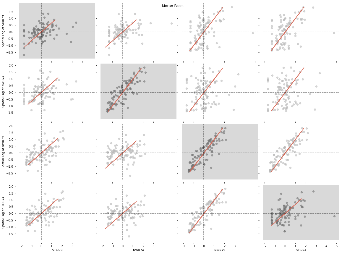
Let's visualise our matrix with splot.esda.moran_facet(). You will see Univariate Moran objects with a grey background, surrounded by all possible bivariate combinations of your input dataset:
from splot.esda import moran_facet

moran_facet(matrix)
plt.show()
Additionally, it is possible to generte your Moran_BV_matrix and a moran_facet using a pandas or geopandas DataFrame as input. Let's have a look at a simple example examining columbus.shp example data:
path = examples.get_path('columbus.shp')
gdf = gpd.read_file(path)
In order for moran_facet to generate sensible results, it is recommended to extract all columns you would specifically like to analyse and generate a new GeoDataFrame:
variables2 = gdf[['HOVAL', 'CRIME', 'INC', 'EW']]
variables2.head()
variables2.shape
We will now generate our own spatial weights leveraging libpysal and create a second matrix2 from our GeoDataFrame. Note that there is no list of varnames needed, this list will be automatically extracted from teh first row of your gdf:
w2 = Queen.from_shapefile(path)
w2
from esda.moran import Moran_BV_matrix

matrix2 = Moran_BV_matrix(variables2, w2)
matrix2
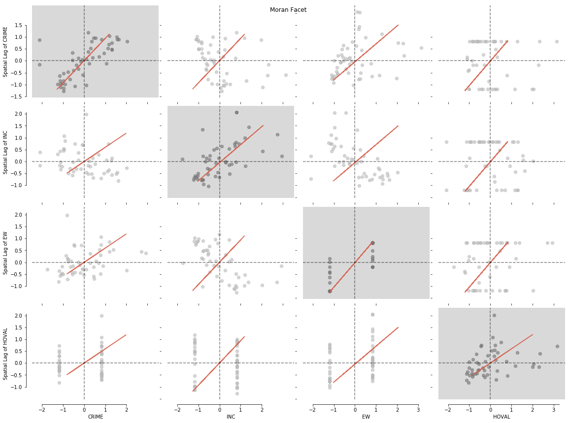
Like in the first example we can now plot our data with a simple splot call:
from splot.esda import moran_facet

moran_facet(matrix2)
plt.show()