
Using the sampler
spvcm is a generic gibbs sampling framework for spatially-correlated variance components models. The current supported models are:
spvcm.bothcontains specifications with correlated errors in both levels, with the first statementse/smadescribing the lower level and the second statementse/smadescribing the upper level. In addition,MVCM, the multilevel variance components model with no spatial correlation, is in thebothnamespace.spvcm.lowercontains two specifications,se/sma, that can be used for a variance components model with correlated lower-level errors.spvcm.uppercontains two specifications,se/smathat can be used for a variance components model with correlated upper-level errors.
Specification
These derive from a variance components specification:
$$ Y \sim \mathcal{N}(X\beta, \Psi_1(\lambda, \sigma^2) + \Delta\Psi_2(\rho, \tau^2)\Delta') $$Where:
- $\beta$, called
Betasin code, is the marginal effect parameter. In this implementation, any region-level covariates $Z$ get appended to the end of $X$. So, if $X$ is $n \times p$ ($n$ observations of $p$ covariates) and $Z$ is $J \times p'$ ($p'$ covariates observed for $J$ regions), then the model's $X$ matrix is $n \times (p + p')$ and $\beta$ is $p + p' \times 1$. - $\Psi_1$ is the covariance function for the response-level model. In the software, a separable covariance is assumed, so that $\Psi_1(\rho, \sigma^2) = \Psi_1(\rho) * I \sigma^2)$, where $I$ is the $n \times n$ covariance matrix. Thus, $\rho$ is the spatial autoregressive parameter and $\sigma^2$ is the variance parameter. In the software, $\Psi_1$ takes any of the following forms:
- Spatial Error (
SE): $\Psi_1(\rho) = [(I - \rho \mathbf{W})'(I - \rho \mathbf{W})]^{-1} \sigma^2$ - Spatial Moving Average (
SMA): $\Psi_1(\rho) = (I + \rho \mathbf{W})(I + \lambda \mathbf{W})'$ - Identity: $\Psi_1(\rho) = I$
- Spatial Error (
- $\Psi_2$ is the region-level covariance function, with region-level autoregressive parameter $\lambda$ and region-level variance $\tau^2$. It has the same potential forms as $\Psi_1$.
- $\alpha$, called
Alphasin code, is the region-level random effect. In a variance components model, this is interpreted as a random effect for the upper-level. For a Varying-intercept format, this random component should be added to a region-level fixed effect to provide the varying intercept. This may also make it more difficult to identify the spatial parameter.
Softare implementation
All of the possible combinations of Spatial Moving Average and Spatial Error processes are contained in the following classes. I will walk through estimating one below, and talk about the various features of the package.
First, the API of the package is defined by the spvcm.api submodule. To load it, use import spvcm.api as spvcm:
import spvcm as spvcm #package API
spvcm.both_levels.Generic # abstract customizable class, ignores rho/lambda, equivalent to MVCM
spvcm.both_levels.MVCM # no spatial effect
spvcm.both_levels.SESE #  both spatial error (SE)
spvcm.both_levels.SESMA # response-level SE, region-level spatial moving average
spvcm.both_levels.SMASE # response-level SMA, region-level SE
spvcm.both_levels.SMASMA # both levels SMA
spvcm.upper_level.Upper_SE # response-level uncorrelated, region-level SE
spvcm.upper_level.Upper_SMA # response-level uncorrelated, region-level SMA
spvcm.lower_level.Lower_SE # response-level SE, region-level uncorrelated
spvcm.lower_level.Lower_SMA # response-level SMA, region-level uncorrelated
Depending on the structure of the model, you need at least:
X, data at the response (lower) levelY, system response in the lower levelmembershiporDelta, the membership vector relating each observation to its group or the "dummy variable" matrix encoding the same information.
Then, if spatial correlation is desired, M is the "upper-level" weights matrix and W the lower-level weights matrix.
Any upper-level data should be passed in $Z$, and have $J$ rows. To fit a varying-intercept model, include an identity matrix in $Z$. You can include state-level and response-level intercept terms simultaneously.
Finally, there are many configuration and tuning options that can be passed in at the start, or assigned after the model is initialized.
First, though, let's set up some data for a model on southern counties predicting HR90, the Homicide Rate in the US South in 1990, using the the percent of the labor force that is unemployed (UE90), a principal component expressing the population structure (PS90), and a principal component expressing resource deprivation.
We will also use the state-level average percentage of families below the poverty line and the average Gini coefficient at the state level for a $Z$ variable.
#seaborn is required for the traceplots
import pysal as ps
import numpy as np
import pandas as pd
import seaborn as sns
import matplotlib.pyplot as plt
import geopandas as gpd
%matplotlib inline
Reading in the data, we'll extract these values we need from the dataframe.
data = ps.pdio.read_files(ps.examples.get_path('south.shp'))
gdf = gpd.read_file(ps.examples.get_path('south.shp'))
data = data[data.STATE_NAME != 'District of Columbia']
X = data[['UE90', 'PS90', 'RD90']].values
N = X.shape[0]
Z = data.groupby('STATE_NAME')[['FP89', 'GI89']].mean().values
J = Z.shape[0]

Y = data.HR90.values.reshape(-1,1)
Then, we'll construct some queen contiguity weights from the files to show how to run a model.
W2 = ps.queen_from_shapefile(ps.examples.get_path('us48.shp'),
                             idVariable='STATE_NAME')
W2 = ps.w_subset(W2, ids=data.STATE_NAME.unique().tolist()) #only keep what's in the data
W1 = ps.queen_from_shapefile(ps.examples.get_path('south.shp'),
                             idVariable='FIPS')
W1 = ps.w_subset(W1, ids=data.FIPS.tolist()) #again, only keep what's in the data

W1.transform = 'r'
W2.transform = 'r'
With the data, upper-level weights, and lower-level weights, we can construct a membership vector or a dummy data matrix. For now, I'll create the membership vector.
membership = data.STATE_NAME.apply(lambda x: W2.id_order.index(x)).values
But, we could also build the dummy variable matrix using pandas, if we have a suitable categorical variable:
Delta_frame = pd.get_dummies(data.STATE_NAME)
Delta = Delta_frame.values
Every call to the sampler is of the following form:
sampler(Y, X, W, M, Z, membership, Delta, n_samples, **configuration)
Where W, M are passed if appropriate, Z is passed if used, and only one of membership or Delta is required. In the end, Z is appended to X, so the effects pertaining to the upper level will be at the tail end of the $\beta$ effects vector. If both Delta and membership are supplied, they're verified against each other to ensure that they agree before they are used in the model.
For all models, the membership vector or an equivalent dummy variable matrix is required. For models with correlation in the upper level, only the upper-level weights matrix $\mathbf{M}$ is needed. For lower level models, the lower-level weights matrix $\mathbf{W}$ is required. For models with correlation in both levels, both $\mathbf{W}$ and $\mathbf{M}$ are required.
Every sampler uses, either in whole or in part, spvcm.both.generic, which implements the full generic sampler discussed in the working paper. For efficiency, the upper-level samplers modify this runtime to avoid processing the full lower-level covariance matrix.
Like many of the R packages dedicated to bayesian models, configuration occurs by passing the correct dictionary to the model call. In addition, you can "setup" the model, configure it, and then run samples in separate steps.
The most common way to call the sampler is something like:
vcsma = spvcm.upper_level.Upper_SMA(Y, X, M=W2, Z=Z,
                                    membership=membership,
                                    n_samples=5000,
                                    configs=dict(tuning=1000,
                                                 adapt_step=1.01))
This model, spvcm.upper_level.Upper_SMA, is a variance components/varying intercept model with a state-level SMA-correlated error.
Thus, there are only five parameters in this model, since $\rho$, the lower-level autoregressive parameter, is constrained to zero:
vcsma.trace.varnames
The results and state of the sampler are stored within the vcsma object. I'll step through the most important parts of this object.
trace
The quickest way to get information out of the model is via the trace object. This is where the results of the tracked parameters are stored each iteration. Any variable in the sampler state can be added to the tracked params. Trace objects are essentially dictionaries with the keys being the name of the tracked parameter and the values being a list of each iteration's sampler output.
vcsma.trace.varnames
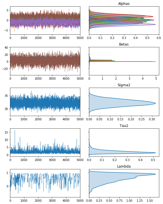
In this case, Lambda is the upper-level moving average parameter, Alphas is the vector of correlated group-level random effects, Tau2 is the upper-level variance, Betas are the marginal effects, and Sigma2 is the lower-level error variance.
I've written two helper functions for working with traces. First is to just dump all the output into a pandas dataframe, which makes it super easy to do work on the samples, or write them out to csv and assess convergence in R's coda package.
trace_dataframe = vcsma.trace.to_df()
the dataframe will have columns containing the elements of the parameters and each row is a single iteration of the sampler:
trace_dataframe.head()
You can write this out to a csv or analyze it in memory like a typical pandas dataframes:
trace_dataframe.mean()
The second is a method to plot the traces:
fig, ax = vcsma.trace.plot()
plt.show()
The trace object can be sliced by (chain, parameter, index) tuples, or any subset thereof.
vcsma.trace['Lambda',-4:] #last 4 draws of lambda
vcsma.trace[['Tau2', 'Sigma2'], 0:2] #the first 2 variance parameters
We only ran a single chain, so the first index is assumed to be zero. You can run more than one chain in parallel, using the builtin python multiprocessing library:
vcsma_p = spvcm.upper_level.Upper_SMA(Y, X, M=W2, Z=Z,
                                      membership=membership,
                                      #run 3 chains
                                      n_samples=5000, n_jobs=3,
                                      configs=dict(tuning=500,
                                                   adapt_step=1.01))
vcsma_p.trace[0, 'Betas', -1] #the last draw of Beta on the first chain.
vcsma_p.trace[1, 'Betas', -1] #the last draw of Beta on the second chain
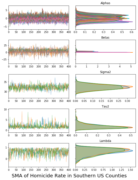
and the chain plotting works also for the multi-chain traces. In addition, there are quite a few traceplot options, and all the plots are returned by the methods as matplotlib objects, so they can also be saved using plt.savefig().
vcsma_p.trace.plot(burn=1000, thin=10)
plt.suptitle('SMA of Homicide Rate in Southern US Counties', y=0, fontsize=20)
#plt.savefig('trace.png') #saves to a file called "trace.png"
plt.show()
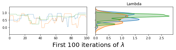
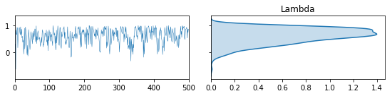
vcsma_p.trace.plot(burn=-100, varnames='Lambda') #A negative burn-in works like negative indexing in Python & R
plt.suptitle('First 100 iterations of $\lambda$', fontsize=20, y=.02)
plt.show() #so this plots Lambda in the first 100 iterations.
To get stuff like posterior quantiles, you can use the attendant pandas dataframe functionality, like describe.
df = vcsma.trace.to_df()
df.describe()
There is also a trace.summarize function that will compute various things contained in spvcm.diagnostics on the chain. It takes a while for large chains, because the statsmodels.tsa.AR estimator is much slower than the ar estimator in R. If you have rpy2 installed and CODA installed in your R environment, I attempt to use R directly.
vcsma.trace.summarize()
So, 5000 iterations, but many parameters have an effective sample size that's much less than this. There's debate about whether it's necesasry to thin these samples in accordance with the effective size, and I think you should thin your sample to the effective size and see if it affects your HPD/Standard Errorrs.
The existing python packages for MCMC diagnostics were incorrect. So, I've implemented many of the diagnostics from CODA, and have verified that the diagnostics comport with CODA diagnostics. One can also use numpy & statsmodels functions. I'll show some types of analysis.
from statsmodels.api import tsa
#if you don't have it, try removing the comment and:
#! pip install statsmodels
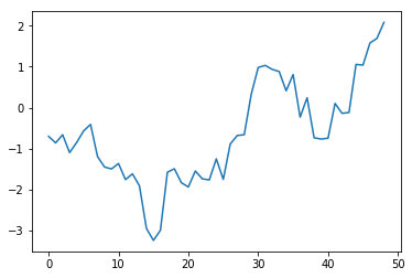
For example, a plot of the partial autocorrelation in $\lambda$, the upper-level spatial moving average parameter, over the last half of the chain is:
plt.plot(tsa.pacf(vcsma.trace['Lambda', -2500:]))
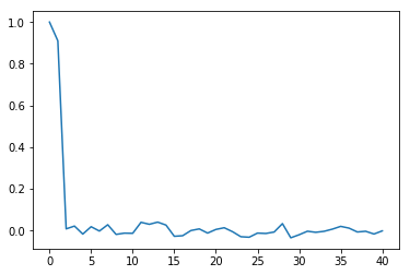
So, the chain is close-to-first order:
tsa.pacf(df.Lambda)[0:3]
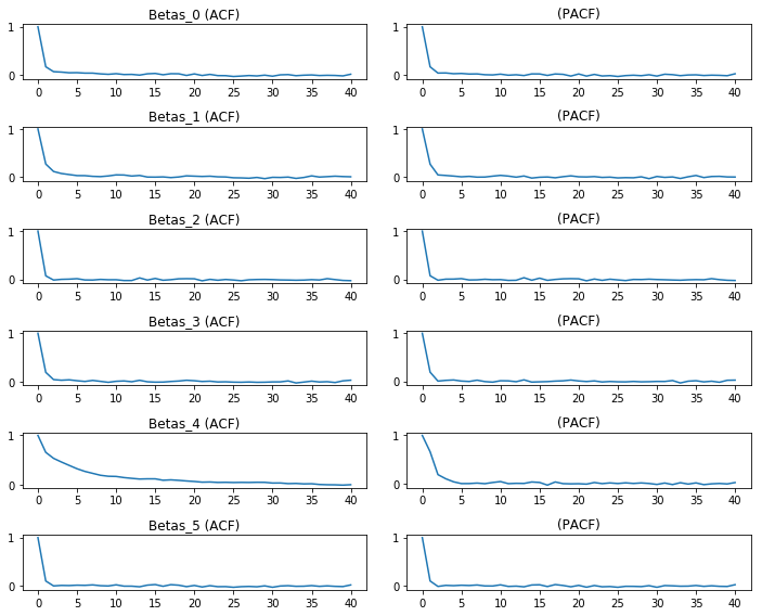
We could do this for many parameters, too. An Autocorrelation/Partial Autocorrelation plot can be made of the marginal effects by:
betas = [c for c in df.columns if c.startswith('Beta')]
f,ax = plt.subplots(len(betas), 2, figsize=(10,8))
for i, col in enumerate(betas):
    ax[i,0].plot(tsa.acf(df[col].values))
    ax[i,1].plot(tsa.pacf(df[col].values)) #the pacf plots take a while
    ax[i,0].set_title(col +' (ACF)')
    ax[i,1].set_title('(PACF)')
f.tight_layout()
plt.show()
As far as the builtin diagnostics for convergence and simulation quality, the diagnostics module exposes a few things:
Geweke statistics for differences in means between chain components:
gstats = spvcm.diagnostics.geweke(vcsma, varnames='Tau2') #takes a while
print(gstats)
Typically, this means the chain is converged at the given "bin" count if the line stays within $\pm2$. The geweke statistic is a test of differences in means between the given chunk of the chain and the remaining chain. If it's outside of +/- 2 in the early part of the chain, you should discard observations early in the chain. If you get extreme values of these statistics throughout, you need to keep running the chain.
plt.plot(gstats[0]['Tau2'][:-1])
We can also compute Monte Carlo Standard Errors like in the mcse R package, which represent the intrinsic error contained in the estimate:
spvcm.diagnostics.mcse(vcsma, varnames=['Tau2', 'Sigma2'])
Another handy statistic is the Partial Scale Reduction factor, which measures of how likely a set of chains run in parallel have converged to the same stationary distribution. It provides the difference in variance between between chains vs. within chains.
If these are significantly larger than one (say, 1.5), the chain probably has not converged. Being marginally below $1$ is fine, too.
spvcm.diagnostics.psrf(vcsma_p, varnames=['Tau2', 'Sigma2'])
Highest posterior density intervals provide a kind of interval estimate for parameters in Bayesian models:
spvcm.diagnostics.hpd_interval(vcsma, varnames=['Betas', 'Lambda', 'Sigma2'])
Sometimes, you want to apply arbitrary functions to each parameter trace. To do this, I've written a map function that works like the python builtin map. For example, if you wanted to get arbitrary percentiles from the chain:
vcsma.trace.map(np.percentile,
                varnames=['Lambda', 'Tau2', 'Sigma2'],
                #arguments to pass to the function go last
                q=[25, 50, 75])
In addition, you can pop the trace results pretty simply to a .csv file and analyze it elsewhere, like if you want to use use the coda Bayesian Diagnostics package in R.
To write out a model to a csv, you can use:
vcsma.trace.to_csv('./model_run.csv')
And, you can even load traces from csvs:
tr = spvcm.abstracts.Trace.from_csv('./model_run.csv')
print(tr.varnames)
tr.plot(varnames=['Tau2'])

vcsma.draw()
And sample steps forward an arbitrary number of times:
vcsma.sample(10)
At this point, we did 5000 initial samples and 11 extra samples. Thus:
vcsma.cycles
Parallel models can suspend/resume sampling too:
vcsma_p.sample(10)
vcsma_p.cycles
Under the hood, it's the draw method that actually ends up calling one run of model._iteration, which is where the actual statistical code lives. Then, it updates all model.traced_params by adding their current value in model.state to model.trace. In addition, model._finalize is called the first time sampling is run, which computes some of the constants & derived quantities that save computing time.
Working with models: state
This is the collection of current values in the sampler. To be efficient, Gibbs sampling must keep around some of the computations used in the simulation, since sometimes the same terms show up in different conditional posteriors. So, the current values of the sampler are stored in state.
All of the following are tracked in the state:
print(vcsma.state.keys())
If you want to track how something (maybe a hyperparameter) changes over sampling, you can pass extra_traced_params to the model declaration:
example = spvcm.upper_level.Upper_SMA(Y, X, M=W2, Z=Z,
                                      membership=membership,
                                      n_samples=250,
                                      extra_traced_params = ['DeltaAlphas'],
                                      configs=dict(tuning=500, adapt_step=1.01))
example.trace.varnames
configs
this is where configuration options for the various MCMC steps are stored. For multilevel variance components models, these are called $\rho$ for the lower-level error parameter and $\lambda$ for the upper-level parameter. Two exact sampling methods are implemented, Metropolis sampling & Slice sampling.
Each MCMC step has its own config:
vcsma.configs
Since vcsma is an upper-level-only model, the Rho config is skipped. But, we can look at the Lambda config. The number of accepted lambda draws is contained in :
vcsma.configs.Lambda.accepted
so, the acceptance rate is
vcsma.configs.Lambda.accepted / float(vcsma.cycles)
Also, if you want to get verbose output from the metropolis sampler, there is a "debug" flag:
example = spvcm.upper_level.Upper_SMA(Y, X, M=W2, Z=Z,
                                      membership=membership,
                                      n_samples=500,
                                      configs=dict(tuning=250,
                                                   adapt_step=1.01,
                                                   debug=True))
Which stores the information about each iteration in a list, accessible from model.configs.<parameter>._cache:
example.configs.Lambda._cache[-1] #let's only look at the last one
Configuration of the MCMC steps is done using the config options dictionary, like done in spBayes in R. The actual configuration classes exist in spvcm.steps:
from spvcm.steps import Metropolis, Slice
Most of the common options are:
Metropolis
jump: the starting standard deviation of the proposal distributiontuning: the number of iterations to tune the scale of the proposalar_low: the lower bound of the target acceptance rate rangear_hi: the upper bound of the target acceptance rate rangeadapt_step: a number (bigger than 1) that will be used to modify the jump in order to keep the acceptance rate betwenar_loandar_hi. Values much larger than1result in much more dramatic tuning.
Slice
width: starting width of the level setadapt: number of previous slices use in the weighted average for the next slice. If0, thewidthis not dynamically tuned.
example = spvcm.upper_level.Upper_SMA(Y, X, M=W2, Z=Z,
                                      membership=membership,
                                      n_samples=500,
                                      configs=dict(tuning=250,
                                                   adapt_step=1.01,
                                      debug=True, ar_low=.1, ar_hi=.4))
example.configs.Lambda.ar_hi, example.configs.Lambda.ar_low
example_slicer = spvcm.upper_level.Upper_SMA(Y, X, M=W2, Z=Z,
                                             membership=membership,
                                             n_samples=500,
                                             configs=dict(Lambda_method='slice'))
example_slicer.trace.plot(varnames='Lambda')
plt.show()
example_slicer.configs.Lambda.adapt, example_slicer.configs.Lambda.width
If you're doing heavy customization, it makes the most sense to first initialize the class without sampling. We did this before when showing how the "extra_traced_params" option worked.
To show, let's initialize a double-level SAR-Error variance components model, but not actually draw anything.
To do this, you pass the option n_samples=0.
vcsese = spvcm.both_levels.SESE(Y, X, W=W1, M=W2, Z=Z,
                                membership=membership,
                                n_samples=0)
This sets up a two-level spatial error model with the default uninformative configuration. This means the prior precisions are all I * .001*, prior means are all 0, spatial parameters are set to -1/(n-1), and prior scale factors are set arbitrarily.
Options are set by assgning to the relevant property in model.configs.
The model configuration object is another dictionary with a few special methods.
Configuration options are stored for each parameter separately:
vcsese.configs
So, for example, if we wanted to turn off adaptation in the upper-level parameter, and fix the Metrpolis jump variance to .25:
vcsese.configs.Lambda.max_tuning = 0
vcsese.configs.Lambda.jump  = .25
Another thing that might be interesting (though not "bayesian") would be to fix the prior mean of $\beta$ to the OLS estimates. One way this could be done would be to pull the Delta matrix out from the state, and estimate:
$$ Y = X\beta + \Delta Z + \epsilon $$
using PySAL:
Delta = vcsese.state.Delta
DeltaZ = Delta.dot(Z)
vcsese.state.Betas_mean0 = ps.spreg.OLS(Y, np.hstack((X, DeltaZ))).betas
If you wanted to start the sampler at a given starting value, you can do so by assigning that value to the Lambda value in state.
vcsese.state.Lambda = -.25
Sometimes, it's suggested that you start the beta vector randomly, rather than at zero. For the parallel sampling, the model starting values are adjusted to induce overdispersion in the start values.
You could do this manually, too:
vcsese.state.Betas += np.random.uniform(-10, 10, size=(vcsese.state.p,1))
Changing the spatial parameter priors is also done by changing their prior in state. This prior must be a function that takes a value of the parameter and return the log of the prior probability for that value.
For example, we could assign P(\lambda) = Beta(2,1) and zero if outside $(0,1)$, and asign $\rho$ a truncated $\mathcal{N}(0,.5)$ prior by first defining their functional form:
from scipy import stats
def Lambda_prior(val):
    if (val < 0) or (val > 1):
        return -np.inf
    return np.log(stats.beta.pdf(val, 2,1))
def Rho_prior(val):
    if (val > .5) or (val < -.5):
        return -np.inf
    return np.log(stats.truncnorm.pdf(val, -.5, .5, loc=0, scale=.5))
And then assigning to their symbols, LogLambda0 and LogRho0 in the state:
vcsese.state.LogLambda0 = Lambda_prior
vcsese.state.LogRho0 = Rho_prior
The efficiency of the sampler is contingent on the lower-level size. If we were to estimate the draw in a dual-level SAR-Error Variance Components iteration:
%timeit vcsese.draw()
To make it easy to work with the model, you can interrupt and resume sampling using keyboard interrupts (ctrl-c or the stop button in the notebook).
%time vcsese.sample(100)
vcsese.sample(10)
Most of the tools in the package are stored in relevant python files in the top level or a dedicated subfolder. Explaining a few:
abstracts.py- the abstract class machinery to iterate over a sampling loop. This is where the classes are defined, likeTrace,Sampler_Mixin, orHashmap.plotting.py- tools for plotting outputsteps.py- the step method definitionsverify.py- likeuserchecks inpysal.spreg, this contains a few sanity checks.utils.py- contains statistical or numerical utilities to make the computation easier, like cholesky multivariate normal sampling, more sparse utility functions, etc.diagnostics.py- all the diagnosticspriors.py- definitions of alternative prior forms. Right now, this is pretty simple.sqlite.py- functions to use a sqlite database instead of an in-memory chain are defined here.
The implementation of a Model
The package is implemented so that every "model type" first sends off to the spvcm.both.Base_Generic, which sets up the state, trace, and priors.
Models are added by writing a model.py file and possibly a sample.py file. The model.py file defines a Base/User class pair (like spreg) that sets up the state and trace. It must define hyperparameters, and can precompute objects used in the sampling loop. The base class should inherit from Sampler_Mixin, which defines all of the machinery of sampling.
The loop through the conditional posteriors should be defined in model.py, in the model._iteration function. This should update the model state in place.
The model may also define a _finalize function which is run once before sampling.
So, if I write a new model, like a varying-intercept model with endogenously-lagged intercepts, I would write a model.py containing something like:
class Base_VISAR(spvcm.generic.Base_Generic):
    def __init__(self, Y, X, M, membership=None, Delta=None,
                 extra_traced_params=None, #record extra things in state
                 n_samples=1000, n_jobs=1, #sampling config
                 priors = None, # dict with prior values for params
                 configs=None, # dict with configs for MCMC steps
                 starting_values=None, # dict with starting values
                 truncation=None, # options to truncate MCMC step priors
                 center=False, # Whether to center the X,Z matrices
                 scale=False # Whether re-scale the X,Z matrices
                 ):
        super(Base_VISAR, self).__init__(self, Y, X, M, W=None,
                                         membership=membership,
                                         Delta=Delta,
                                         n_samples=0, n_jobs=n_jobs,
                                         priors=priors, configs=configs,
                                         starting_values=starting_values,
                                         truncation=truncation,
                                         center=center,
                                         scale=scale
                                         )
        self.sample(n_samples, n_jobs=n_jobs)

        def _finalize(self):
            # the degrees of freedom of the variance parameter is constant
            self.state.Sigma2_an = self.state.N/2 + self.state.Sigma2_a0
            ...

        def _iteration(self):

            # computing the values needed to sample from the conditional posteriors
            mean = spdot(X.T, spdot(self.PsiRhoi, X)) / Sigma2 + self.state.bmean0
            ...
    ...
I've organized the directories in this project into both_levels, upper_level, lower_level, and hierarchical, which contains some of the spatially-varying coefficient models & other models I'm working on that are unrelated to the multilevel variance components stuff.
Since most of the _iteration loop is the same between models, most of the models share the same sampling code, but customize the structure of the covariance in each level. These covariance variables are stored in the state.Psi_1, for the lower-level covariance, and state.Psi_2 for the upper-level covariance. Likewise, the precision functions are state.Psi_1i and state.Psi_2i.
For example:
vcsese.state.Psi_1 #lower-level covariance
vcsese.state.Psi_2 #upper-level covariance
vcsma.state.Psi_2 #upper-level covariance
vcsma.state.Psi_2i
vcsma.state.Psi_1
The functions that generate the covariance matrices are stored in spvcm.utils. They can be arbitrarily overwritten for alternative covariance specifications.
Thus, if we want to sample a model with a new covariance specification, then we need to define functions for the variance and precision.