shortest-path-visualization

If any part of this notebook is used in your research, please cite with the reference found in README.md.

Generating regular lattices and visualizing shortest paths

Creating data for testing and demonstrating routes

Author: James D. Gaboardi jgaboardi@gmail.com

This notebook is a walk-through for:

Instantiating a simple network through a generated regular lattice
Generating shortest path geometric objects
Visualizing shortest paths

%load_ext watermark
%watermark

2020-01-24T19:49:38-05:00

CPython 3.7.3
IPython 7.10.2

compiler   : Clang 9.0.0 (tags/RELEASE_900/final)
system     : Darwin
release    : 19.2.0
machine    : x86_64
processor  : i386
CPU cores  : 4
interpreter: 64bit

In addtion to the base spaghetti requirements (and their dependecies), this notebook requires installations of:

geopandas
- $ conda install -c conda-forge geopandas
matplotlib
- $ conda install matplotlib

import spaghetti
import matplotlib
import matplotlib.pyplot as plt
import libpysal
from libpysal.cg import Point
try:
    from IPython.display import set_matplotlib_formats
    set_matplotlib_formats("retina")
except ImportError:
    pass
%matplotlib inline
%watermark -w
%watermark -iv

watermark 2.0.2
libpysal   4.2.0
matplotlib 3.1.2
spaghetti  1.4.0

1. Demonstration with a synthetic network

1.1 Instantiate a network from a 4x4 regular lattice

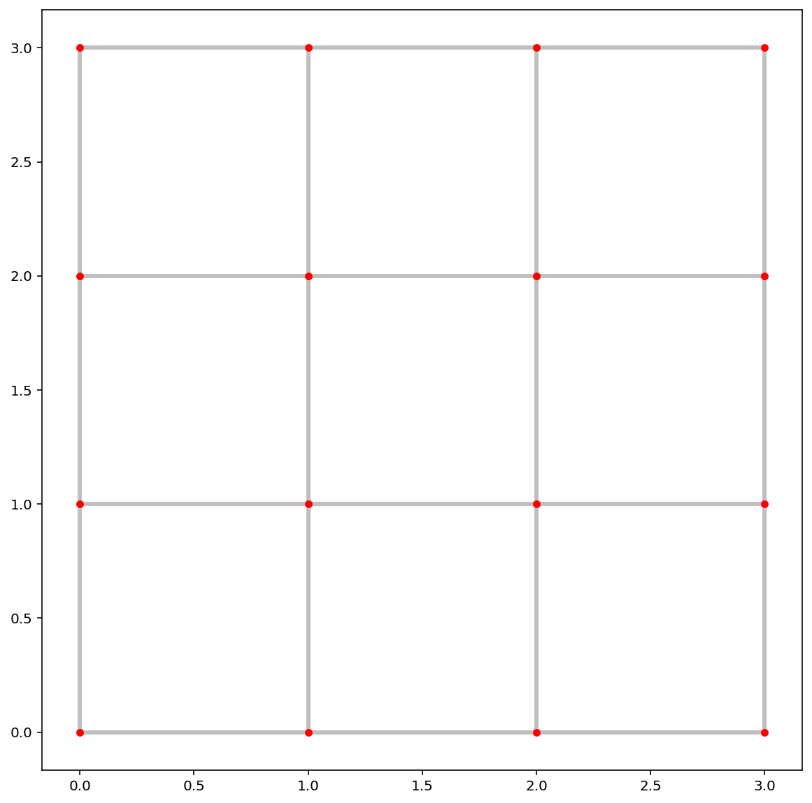
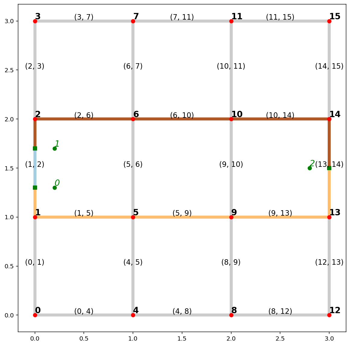
lattice = spaghetti.regular_lattice(4)
ntw = spaghetti.Network(in_data=lattice)

1.2. Extract network elements and visualize them

vertices, arcs = spaghetti.element_as_gdf(ntw, vertices=True, arcs=True)

base = arcs.plot(linewidth=3, alpha=0.25, color="k", zorder=0, figsize=(10, 10))
vertices.plot(ax=base, markersize=20, color="red", zorder=1);

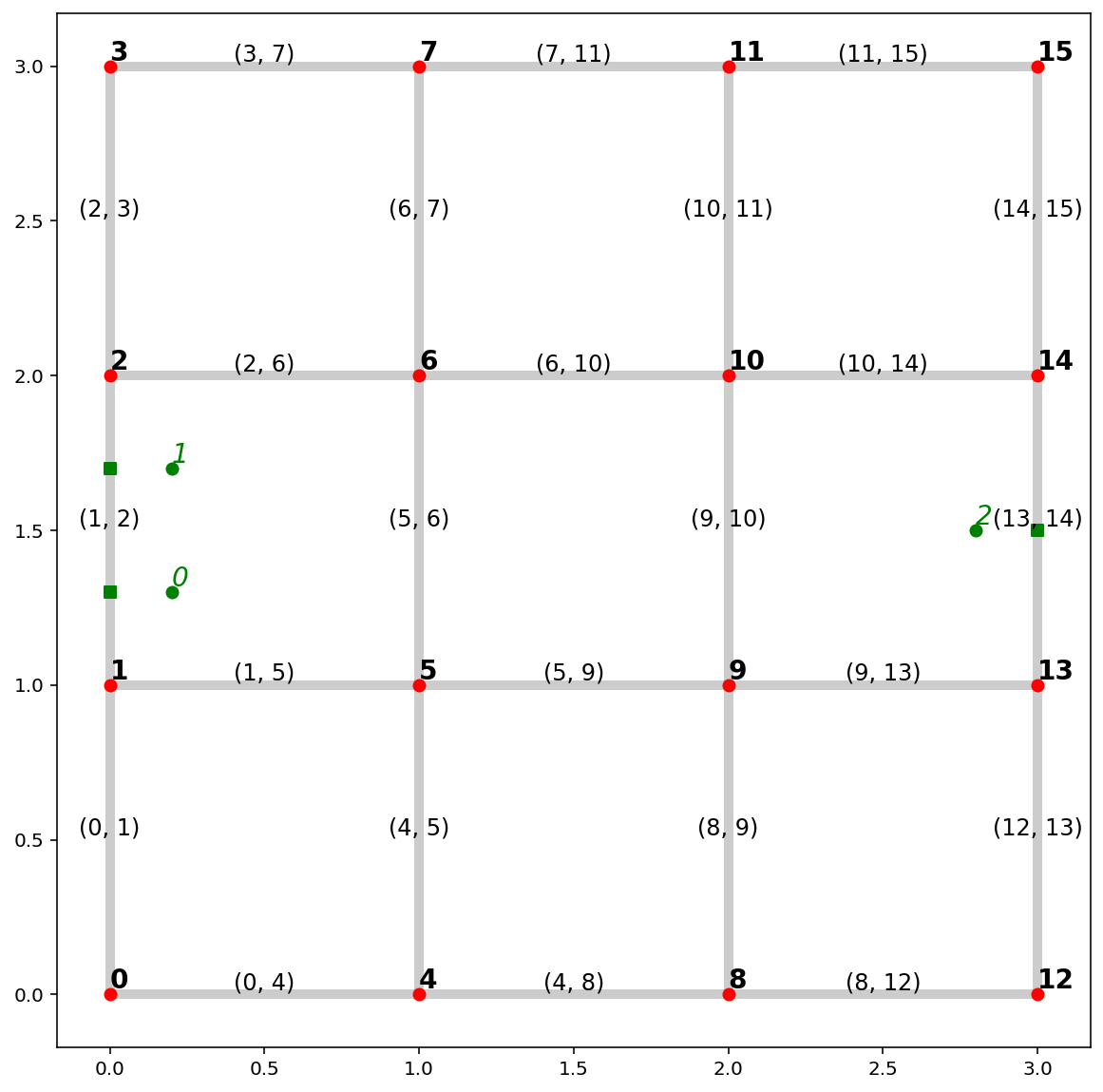
1.3. Instantiate several synthetic observations and snap them to the network

synth_obs = [Point([0.2, 1.3]), Point([0.2, 1.7]), Point([2.8, 1.5])]
ntw.snapobservations(synth_obs, "synth_obs")

1.4. Extract point patterns and visualize plot

Note the labeling for network elements and observations

# true locations of synthetic observations
pp_obs = spaghetti.element_as_gdf(ntw, pp_name="synth_obs")
# snapped locations of synthetic observations
pp_obs_snapped = spaghetti.element_as_gdf(ntw, pp_name="synth_obs", snapped=True)

base = arcs.plot(alpha=0.2, linewidth=5, color="k", figsize=(10, 10), zorder=0)
vertices.plot(ax=base, color="r", zorder=1)
pp_obs.plot(ax=base, color="g", zorder=2)
pp_obs_snapped.plot(ax=base, color="g", marker="s", zorder=2)
# arc labels
arcs.apply(
    lambda x: base.annotate(
        s=x.id, xy=x.geometry.centroid.coords[0], size=12, ha="center", va="bottom"
    ),
    axis=1,
)
# vertex labels
vertices.apply(
    lambda x: base.annotate(
        s=x.id, xy=x.geometry.coords[0], weight="bold", size=14, ha="left", va="bottom"
    ),
    axis=1,
)
# synthetic observation labels
pp_obs.apply(
    lambda x: base.annotate(
        s=x.id,
        xy=x.geometry.coords[0],
        style="oblique",
        color="g",
        size=14,
        ha="left",
        va="bottom",
    ),
    axis=1,
);

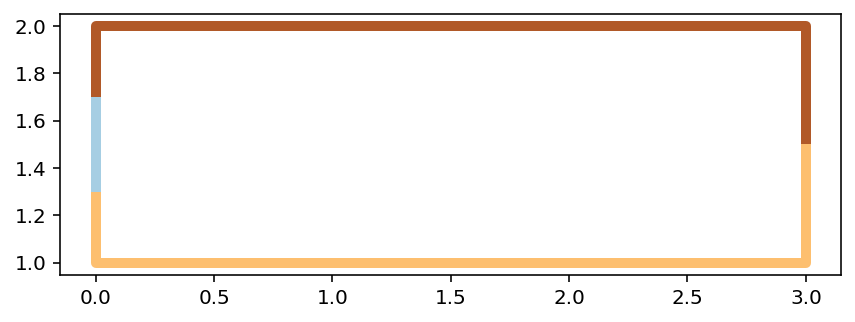
1.5. Generate observation shortest path trees

d2d_dist, tree = ntw.allneighbordistances("synth_obs", gen_tree=True)
d2d_dist

array([[nan, 0.4, 3.8],
       [0.4, nan, 3.8],
       [3.8, 3.8, nan]])

Note that a tag of `(-0.1, -0.1)` labels the points as being snapped to the same network arc

tree

{(0, 1): (-0.1, -0.1), (0, 2): (1, 13), (1, 2): (2, 14)}

1.6. Generate shortest paths as `libpysal.cg.Chain` objects

paths = ntw.shortest_paths(tree, "synth_obs")
paths

{(0, 1): [(0.0, 1.3), (0.0, 1.7)],
 (0, 2): [(0.0, 1.3),
  (0.0, 1.0),
  (1.0, 1.0),
  (2.0, 1.0),
  (3.0, 1.0),
  (3.0, 1.5)],
 (1, 2): [(0.0, 1.7),
  (0.0, 2.0),
  (1.0, 2.0),
  (2.0, 2.0),
  (3.0, 2.0),
  (3.0, 1.5)]}

1.7. Extract the shortest paths within `geopandas.GeoDataFrame` and plot

paths_gdf = spaghetti.element_as_gdf(ntw, routes=paths)
paths_gdf

	id	geometry
0	(0, 1)	LINESTRING (0 1.3, 0 1.7)
1	(0, 2)	LINESTRING (0 1.3, 0 1, 1 1, 2 1, 3 1, 3 1.5)
2	(1, 2)	LINESTRING (0 1.7, 0 2, 1 2, 2 2, 3 2, 3 1.5)

paths_gdf.plot(figsize=(7, 7), column=paths_gdf.index.name, cmap="Paired", linewidth=5);

1.8. Plot the routes within the context of the network

base = arcs.plot(alpha=0.2, linewidth=5, color="k", figsize=(10, 10), zorder=0)
paths_gdf.plot(ax=base, column="id", cmap="Paired", linewidth=5, zorder=1)
vertices.plot(ax=base, color="r", zorder=2)
pp_obs.plot(ax=base, color="g", zorder=3)
pp_obs_snapped.plot(ax=base, color="g", marker="s", zorder=2)
# arc labels
arcs.apply(
    lambda x: base.annotate(
        s=x.id, xy=x.geometry.centroid.coords[0], size=12, ha="center", va="bottom"
    ),
    axis=1,
)
# vertex labels
vertices.apply(
    lambda x: base.annotate(
        s=x.id, xy=x.geometry.coords[0], weight="bold", size=14, ha="left", va="bottom"
    ),
    axis=1,
)
# synthetic observation labels
pp_obs.apply(
    lambda x: base.annotate(
        s=x.id,
        xy=x.geometry.coords[0],
        style="oblique",
        color="g",
        size=14,
        ha="left",
        va="bottom",
    ),
    axis=1,
);

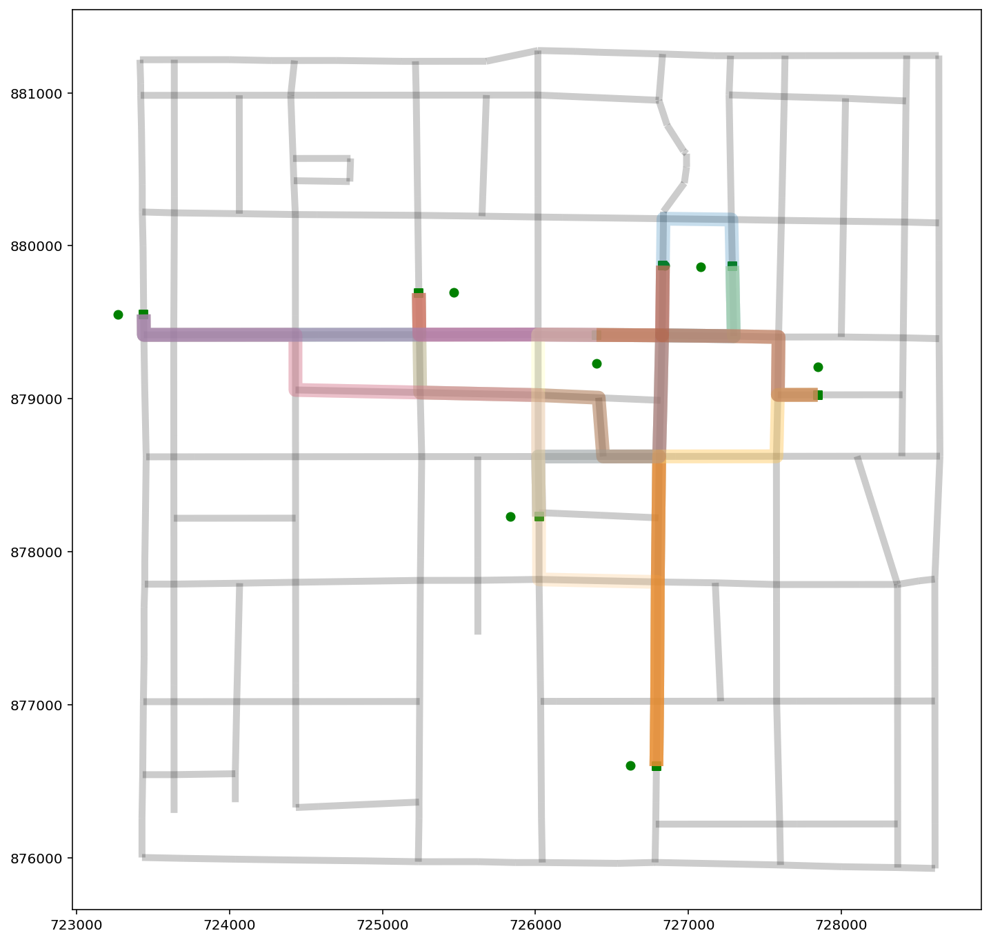
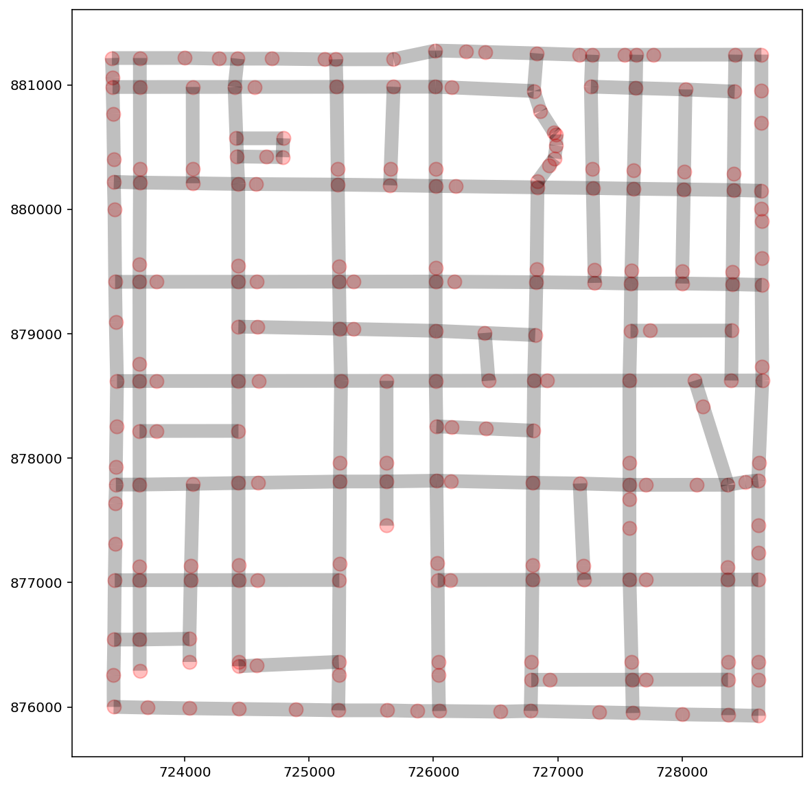
2. Demostration with emprical datasets

2.1 Instantiate an emprical network, extract elements, and visualize

ntw = spaghetti.Network(in_data=libpysal.examples.get_path("streets.shp"))
vertices, arcs = spaghetti.element_as_gdf(ntw, vertices=True, arcs=True)

base = arcs.plot(linewidth=10, alpha=0.25, color="k", figsize=(10, 10))
vertices.plot(ax=base, markersize=100, alpha=0.25, color="red");

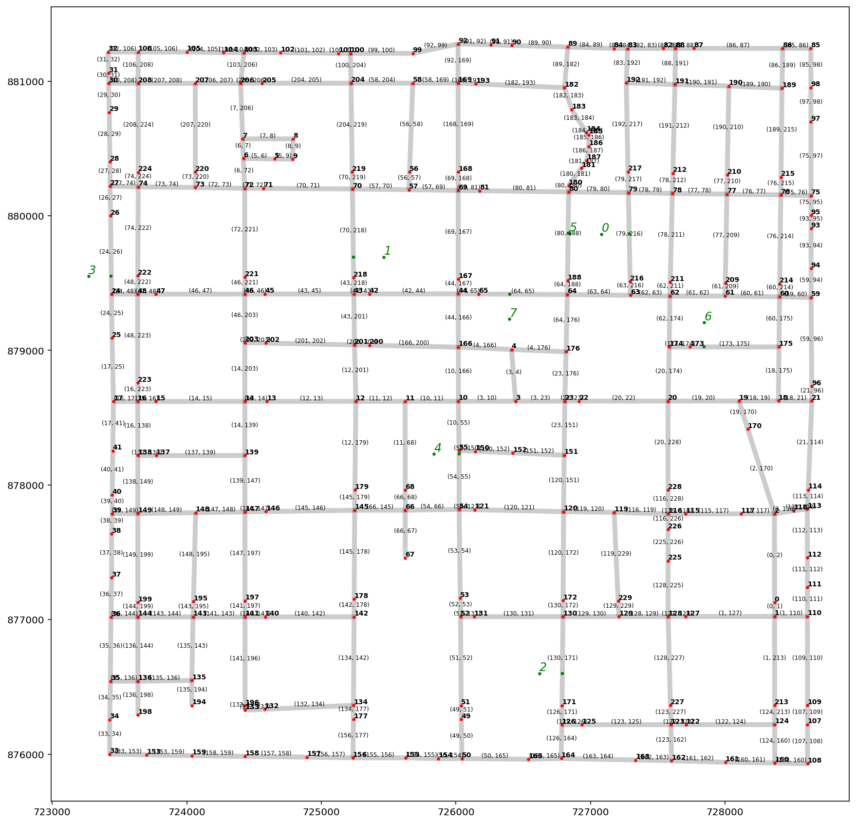
2.2 Snap emprical observations and extract the point patterns as `geopandas.GeoDataFrames`

ntw.snapobservations(libpysal.examples.get_path("schools.shp"), "schools")
pp_obs = spaghetti.element_as_gdf(ntw, pp_name="schools")
pp_obs_snapped = spaghetti.element_as_gdf(ntw, pp_name="schools", snapped=True)

2.3 Plot empirical data

base = arcs.plot(alpha=0.2, linewidth=5, color="k", figsize=(15, 15), zorder=0)
vertices.plot(ax=base, markersize=5, color="r", zorder=1)
pp_obs.plot(ax=base, markersize=5, color="g", zorder=2)
pp_obs_snapped.plot(ax=base, markersize=5, marker="s", color="g", zorder=2)
# arc labels
arcs.apply(
    lambda x: base.annotate(
        s=x.id, xy=x.geometry.centroid.coords[0], size=6, ha="center", va="bottom"
    ),
    axis=1,
)
# vertex labels
vertices.apply(
    lambda x: base.annotate(
        s=x.id, xy=x.geometry.coords[0], weight="bold", size=7, ha="left", va="bottom"
    ),
    axis=1,
)
# school labels
pp_obs.apply(
    lambda x: base.annotate(
        s=x.id,
        xy=x.geometry.coords[0],
        style="oblique",
        color="g",
        size=12,
        ha="left",
        va="bottom",
    ),
    axis=1,
);

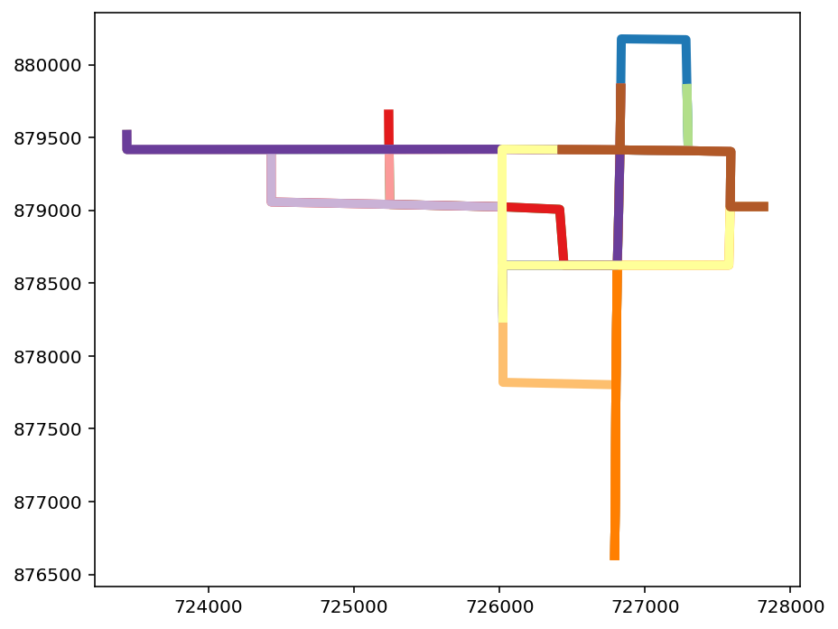
2.4 Generate shortest path routes and extract them

d2d_dist, tree = ntw.allneighbordistances("schools", gen_tree=True)
paths = ntw.shortest_paths(tree, "schools")
paths_gdf = spaghetti.element_as_gdf(ntw, routes=paths)
paths_gdf.head()

	id	geometry
0	(0, 1)	LINESTRING (727287.664 879867.386, 727294.797 ...
1	(0, 2)	LINESTRING (727287.664 879867.386, 727294.797 ...
2	(0, 3)	LINESTRING (727287.664 879867.386, 727294.797 ...
3	(0, 4)	LINESTRING (727287.664 879867.386, 727294.797 ...
4	(0, 5)	LINESTRING (727287.664 879867.386, 727281.557 ...

2.5 Plot the shortest path routes

paths_gdf.plot(figsize=(7, 7), column=paths_gdf.index.name, cmap="Paired", linewidth=5);

2.6. Plot the routes within the context of the network

base = arcs.plot(alpha=0.2, linewidth=5, color="k", figsize=(12, 12), zorder=0)
pp_obs.plot(ax=base, color="g", zorder=2)
pp_obs_snapped.plot(ax=base, color="g", marker="s", zorder=2)
paths_gdf.plot(ax=base, column="id", cmap="Paired", linewidth=10, alpha=0.25);