
This is an example of the PySAL segregation framework to perform inference on a single value and comparative inference using simulations under the null hypothesis. Once the segregation classes are fitted, the user can perform inference to shed light for statistical significance in regional analysis. Currently, it is possible to make inference for a single measure or for two values of the same measure.
The summary of the inference wrappers is presented in the following Table:
| Inference Type | Class/Function | Function main Inputs | Function Outputs |
|---|---|---|---|
| Single Value | SingleValueTest | seg_class, iterations_under_null, null_approach, two_tailed | p_value, est_sim, statistic |
| Two Value | TwoValueTest | seg_class_1, seg_class_2, iterations_under_null, null_approach | p_value, est_sim, est_point_diff |
Firstly let's import the module/functions for the use case:
%matplotlib inline

import geopandas as gpd
import segregation
import libpysal
import pandas as pd
import numpy as np

from segregation.inference import SingleValueTest, TwoValueTest
Then it's time to load some data to estimate segregation. We use the data of 2000 Census Tract Data for the metropolitan area of Sacramento, CA, USA.
We use a geopandas dataframe available in PySAL examples repository.
For more information about the data: https://github.com/pysal/libpysal/tree/master/libpysal/examples/sacramento2
s_map = gpd.read_file(libpysal.examples.get_path("sacramentot2.shp"))
s_map.columns
gdf = s_map[['geometry', 'HISP_', 'TOT_POP']]
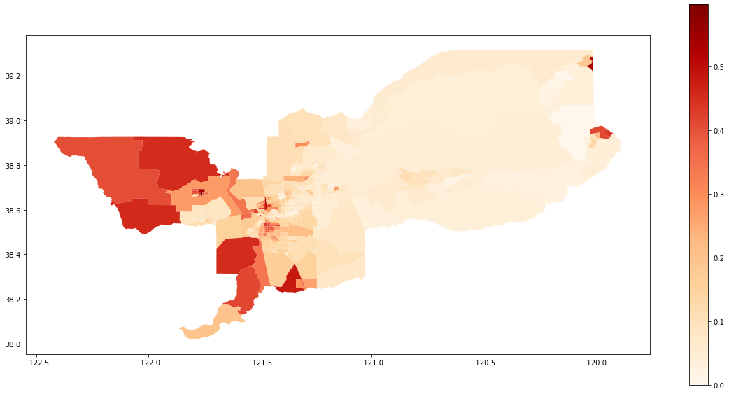
We also can plot the spatial distribution of the composition of the Hispanic population over the tracts of Sacramento:
gdf['composition'] = gdf['HISP_'] / gdf['TOT_POP']

gdf.plot(column = 'composition',
         cmap = 'OrRd',
         figsize=(20,10),
         legend = True)
The SingleValueTest function expect to receive a pre-fitted segregation class and then it uses the underlying data to iterate over the null hypothesis and comparing the results with point estimation of the index. Thus, we need to firstly estimate some measure. We can fit the classic Dissimilarity index:
from segregation.aspatial import Dissim
D = Dissim(gdf, 'HISP_', 'TOT_POP')
D.statistic
The question that may rise is "Is this value of 0.32 statistically significant under some pre-specified circumstance?". To answer this, it is possible to rely on the Infer_Segregation function to generate several values of the same index (in this case the Dissimilarity Index) under the hypothesis and compare them with the one estimated by the dataset of Sacramento. To generate 1000 values assuming evenness, you can run:
infer_D_eve = SingleValueTest(D, iterations_under_null = 1000, null_approach = "evenness", two_tailed = True)
This class has a quick plotting method to inspect the generated distribution with the estimated value from the sample (vertical red line):
infer_D_eve.plot()
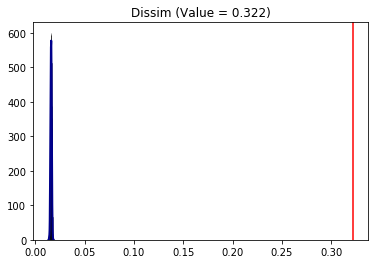
It is possible to see that clearly the value of 0.3218 is far-right in the distribution indicating that the hispanic group is, indeed, significantly segregated in terms of the Dissimilarity index under evenness. You can also check the mean value of the distribution using the est_sim attribute which represents all the D draw from the simulations:
infer_D_eve.est_sim.mean()
The two-tailed p-value of the following hypothesis test:
$$H_0: under \ evenness, \ Sacramento \ IS \ NOT \ segregated \ in \ terms \ of \ the \ Dissimilarity \ index \ (D)$$$$H_1: under \ evenness, \ Sacramento \ IS \ segregated \ in \ terms \ of \ the \ Dissimilarity \ index \ (D)$$can be accessed with the p_value attribute:
infer_D_eve.p_value
Therefore, we can conclude that Sacramento is statistically segregated at 5% of significance level (p.value < 5%) in terms of D.
You can also test under different approaches for the null hypothesis:
infer_D_sys = SingleValueTest(D, iterations_under_null = 5000, null_approach = "systematic", two_tailed = True)
infer_D_sys.plot()
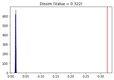
The conclusions are analogous as the evenness approach.
The Infer_Segregation wrapper can handle any class of the PySAL segregation module. It is possible to use it in the Relative Concentration (RCO) segregation index:
from segregation.spatial import RelativeConcentration
RCO = RelativeConcentration(gdf, 'HISP_', 'TOT_POP')
Since RCO is an spatial index (i.e. depends on the spatial context), it makes sense to use the permutation null approach. This approach relies on randomly allocating the sample values over the spatial units and recalculating the chosen index to all iterations.
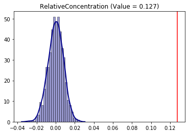
infer_RCO_per = SingleValueTest(RCO, iterations_under_null = 1000, null_approach = "permutation", two_tailed = True)
infer_RCO_per.plot()
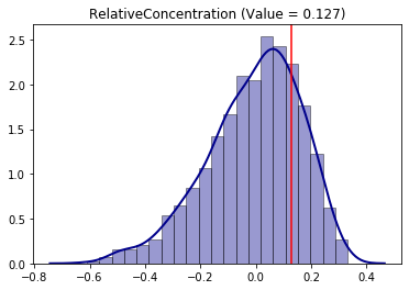
infer_RCO_per.p_value
Analogously, the conclusion for the Relative Concentration index is that Sacramento is not significantly (under 5% of significance, because p-value > 5%) concentrated for the hispanic people.
Additionaly, it is possible to combine the null approaches establishing, for example, a permutation along with evenness of the frequency of the Sacramento hispanic group. With this, the conclusion of the Relative Concentration changes.
infer_RCO_eve_per = SingleValueTest(RCO, iterations_under_null = 1000, null_approach = "even_permutation", two_tailed = True)
infer_RCO_eve_per.plot()
Using the same permutation approach for the Relative Centralization (RCE) segregation index:
from segregation.spatial import RelativeCentralization
RCE = RelativeCentralization(gdf, 'HISP_', 'TOT_POP')
infer_RCE_per = SingleValueTest(RCE, iterations_under_null = 1000, null_approach = "permutation", two_tailed = True)
infer_RCE_per.plot()
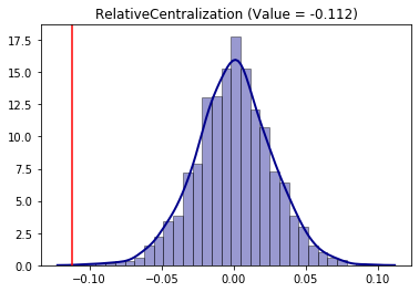
The conclusion is that the hispanic group is negatively significantly (as the point estimation is in the left side of the distribution) in terms of centralization. This behavior can be, somehow, inspected in the map as the composition tends to be more concentraded outside of the center of the overall region.
To compare two different values, the user can rely on the TwoValueTest function. Similar to the previous function, the user needs to pass two segregation SM classes to be compared, establish the number of iterations under null hypothesis with iterations_under_null, specify which type of null hypothesis the inference will iterate with null_approach argument and, also, can pass additional parameters for each segregation estimation.
Obs.: in this case, each measure has to be the same class as it would not make much sense to compare, for example, a Gini index with a Delta index
This example uses all census data that the user must provide your own copy of the external database. A step-by-step procedure for downloading the data can be found here: https://github.com/spatialucr/geosnap/blob/master/examples/01_getting_started.ipynb. After the user download the zip files, you must provide the path to these files.
import os
#os.chdir('path_to_zipfiles')
import geosnap
from geosnap.data.data import read_ltdb

sample = "LTDB_Std_All_Sample.zip"
full = "LTDB_Std_All_fullcount.zip"

read_ltdb(sample = sample, fullcount = full)

df_pre = geosnap.data.db.ltdb
df_pre.head()
In this example, we are interested to assess the comparative segregation of the non-hispanic black people in the census tracts of the Riverside, CA, county between 2000 and 2010. Therefore, we extract the desired columns and add some auxiliary variables:
df = df_pre[['n_nonhisp_black_persons', 'n_total_pop', 'year']]

df['geoid'] = df.index
df['state'] = df['geoid'].str[0:2]
df['county'] = df['geoid'].str[2:5]
df.head()
Filtering Riverside County and desired years of the analysis:
df_riv = df[(df['state'] == '06') & (df['county'] == '065') & (df['year'].isin(['2000', '2010']))]
df_riv.head()
Merging it with desired map.
map_url = 'https://raw.githubusercontent.com/renanxcortes/inequality-segregation-supplementary-files/master/Tracts_grouped_by_County/06065.json'
map_gpd = gpd.read_file(map_url)
gdf = map_gpd.merge(df_riv,
                    left_on = 'GEOID10',
                    right_on = 'geoid')[['geometry', 'n_nonhisp_black_persons', 'n_total_pop', 'year']]

gdf['composition'] = np.where(gdf['n_total_pop'] == 0, 0, gdf['n_nonhisp_black_persons'] / gdf['n_total_pop'])
gdf.head()
gdf_2000 = gdf[gdf.year == 2000]
gdf_2010 = gdf[gdf.year == 2010]
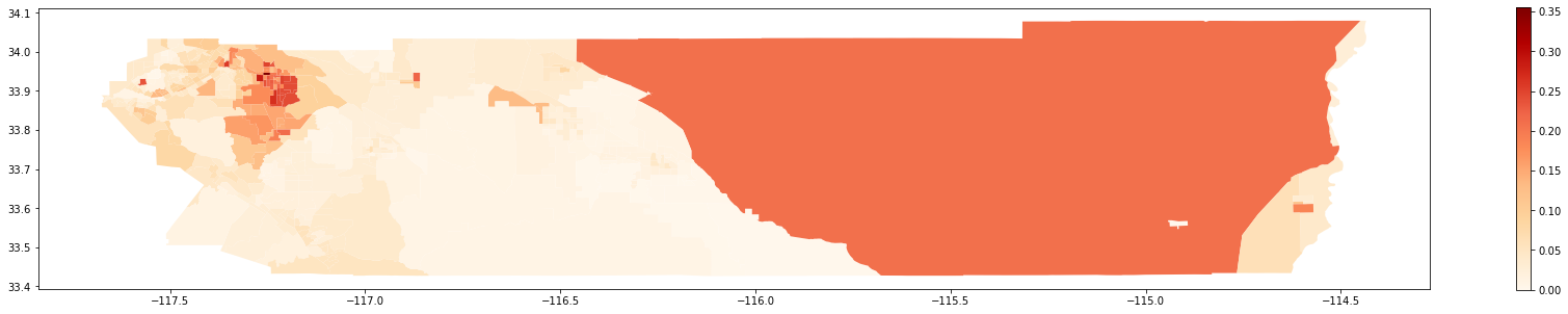
Map of 2000:
gdf_2000.plot(column = 'composition',
              cmap = 'OrRd',
              figsize = (30,5),
              legend = True)
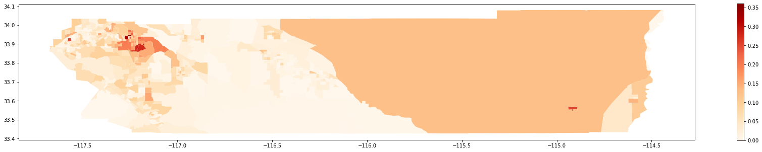
Map of 2010:
gdf_2010.plot(column = 'composition',
              cmap = 'OrRd',
              figsize = (30,5),
              legend = True)
A question that may rise is "Was it more or less segregated than 2000?". To answer this, we rely on simulations to test the following hypothesis:
$$H_0: Segregation\ Measure_{2000} - Segregation\ Measure_{2010} = 0$$D_2000 = Dissim(gdf_2000, 'n_nonhisp_black_persons', 'n_total_pop')
D_2010 = Dissim(gdf_2010, 'n_nonhisp_black_persons', 'n_total_pop')
D_2000.statistic - D_2010.statistic
We can see that Riverside was more segregated in 2000 than in 2010. But, was this point difference statistically significant? We use the random_label approach which consists in random labelling the data between the two periods and recalculating the Dissimilarity statistic (D) in each iteration and comparing it to the original value.
compare_D_fit = TwoValueTest(D_2000, D_2010, iterations_under_null = 1000, null_approach = "random_label")
The TwoValueTest class also has a plotting method:
compare_D_fit.plot()
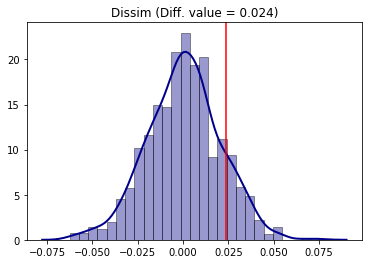
To access the two-tailed p-value of the test:
compare_D_fit.p_value
The conclusion is that, for the Dissimilarity index and 5% of significance, segregation in Riverside was not different between 2000 and 2010 (since p-value > 5%).
Analogously, the same steps can be made for the Gini segregation index.
from segregation.aspatial import GiniSeg
G_2000 = GiniSeg(gdf_2000, 'n_nonhisp_black_persons', 'n_total_pop')
G_2010 = GiniSeg(gdf_2010, 'n_nonhisp_black_persons', 'n_total_pop')
compare_G_fit = TwoValueTest(G_2000, G_2010, iterations_under_null = 1000, null_approach = "random_label")
compare_G_fit.plot()
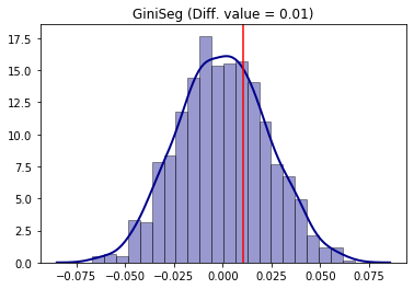
The absence of significance is also present as the point estimation of the difference (vertical red line) is located in the middle of the distribution of the null hypothesis simulated.
As an example of a spatial index, comparative inference can be performed for the Spatial Dissimilarity Index (SD). For this, we use the counterfactual_composition approach as an example.
In this framework, the population of the group of interest in each unit is randomized with a constraint that depends on both cumulative density functions (cdf) of the group of interest composition to the group of interest frequency of each unit. In each unit of each iteration, there is a probability of 50\% of keeping its original value or swapping to its corresponding value according of the other composition distribution cdf that it is been compared against.
from segregation.spatial import SpatialDissim
SD_2000 = SpatialDissim(gdf_2000, 'n_nonhisp_black_persons', 'n_total_pop')
SD_2010 = SpatialDissim(gdf_2010, 'n_nonhisp_black_persons', 'n_total_pop')
compare_SD_fit = TwoValueTest(SD_2000, SD_2010, iterations_under_null = 500, null_approach = "counterfactual_composition")
compare_SD_fit.plot()
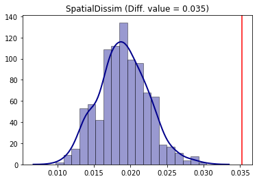
The conclusion is that for the Spatial Dissimilarity index under this null approach, the year of 2000 was more segregated than 2010 for the non-hispanic black people in the region under study.