Table of Contents

• PySAL segregation module for spatial indexes
  • Notation
    • Spatial Dissimilarity
    • Boundary Spatial Dissimilarity
    • Perimeter/Area Ratio Spatial Dissimilarity
    • Spatial Proximity Profile
    • Spatial Proximity
    • Absolute Clustering
    • Relative Clustering
    • Distance Decay Isolation
    • Distance Decay Exposure
    • Delta
    • Absolute Concentration
    • Relative Concentration
    • Absolute Centralization and Relative Centralization
    • Spatial Minimum-Maximum Index (SMM)

PySAL segregation module for spatial indexes

This is an example notebook of functionalities for spatial indexes of the segregation module. Firstly, we need to import the packages we need.

Then it's time to load some data to estimate segregation. We use the data of 2000 Census Tract Data for the metropolitan area of Sacramento, CA, USA.

We use a geopandas dataframe available in PySAL examples repository.

For more information about the data: https://github.com/pysal/libpysal/tree/master/libpysal/examples/sacramento2

The data have several demographic variables. We are going to assess the segregation of the Hispanic Population (variable 'HISP_'). For this, we only extract some columns of the geopandas dataframe.

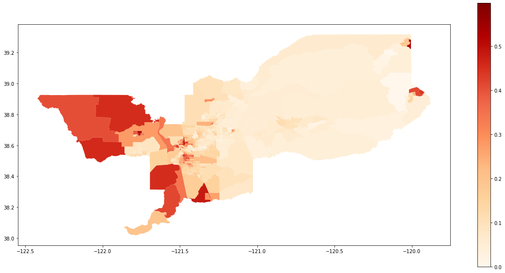
We also can plot the spatial distribution of the composition of the Hispanic population over the tracts of Sacramento:

Notation

For consistency of notation, we assume that $n_{ij}$ is the population of unit $i \in \{1, ..., I\}$ of group $j \in \{x, y\}$, also $\sum_{j}n_{ij} = n_{i.}$, $\sum_{i}n_{ij} = n_{.j}$, $\sum_{i}\sum_{j}n_{ij} = n_{..}$, $\tilde{s}_{ij} = \frac{n_{ij}}{n_{i.}}$, $\hat{s}_{ij} = \frac{n_{ij}}{n_{.j}}$. The segregation indexes can be build for any group $j$ of the data.

Spatial Dissimilarity

The Dissimilarity Index (D) is given by:

$$ D=\sum_{i=1}^{I}\frac{n_{i.}\mid \tilde{s}_{ij}-\frac{n_{.j}}{n_{..}}\mid}{2n_{..}\frac{n_{.j}}{n_{..}}\left ( 1-\frac{n_{.j}}{n_{..}} \right ).} $$

The Spatial Dissimilarity (SD) is given by:

$$ SD = D-\frac{\sum_{i_1=1}^{I}\sum_{i_2=1}^{I}\left | \tilde{s}_{ij}^{i_1}-\tilde{s}_{ij}^{i_2} \right |c_{i_1i_2}}{\sum_{i_1=1}^{I}\sum_{i_2=1}^{I}c_{i_1i_2}} $$

where $\tilde{s}_{ij}^{i_1}$ and $\tilde{s}_{ij}^{i_2}$ are the proportions of the minority population in the units $i_1$ and $i_2$, respectively and where $c_{i_1i_2}$ denotes an element at $(i_1,i_2)$ in a matrix C, which becomes one only if $i_1$ and $i_2$ are considered neighbors.

The index is fitted below:

All the segregation classes have the statistic and the core_data attributes. We can access the point estimation of SD for the data set with the statistic attribute:

Boundary Spatial Dissimilarity

The boundary spatial D (BSD) is given by:

$$ BSD = D - \frac{1}{2}{\sum_{i_1=1}^{I}\sum_{i_2=1}^{I}w_{i_1i_2} \left | \tilde{s}_{ij}^{i_1} - \tilde{s}_{ij}^{i_2} \right |} $$

where

$$ w_{i_1i_2} = \frac{cb_{i_1i_2}}{\sum_{i_2=1}^{I}d_{i_1i_2}} $$

where $\tilde{s}_{ij}^{i_1}$ and $\tilde{s}_{ij}^{i_2}$ are the proportions of the minority population in the units $i_1$ and $i_2$, respectively, and $cb_{i_1i_2}$ is the length of the common boundary of areal units $i_1$ and $i_2$.

The index is fitted below:

Perimeter/Area Ratio Spatial Dissimilarity

The perimeter/area ratio Spatial D (PARD) is a spatial dissimilarity index that takes into consideration the perimeter and the area of each unit by adding a specific multiplicative term in the second term of BSD (the spatial effect):

$$ \frac{\frac{1}{2}\left [\left ( \frac{P_i}{A_i} \right )+\left ( \frac{P_j}{A_j} \right ) \right ]}{MAX\left ( \frac{P}{A} \right )} $$

where $P_i$ and $A_i$ are the perimeter and area of unit $i$, respectively and $MAX(P/A)$ is the maximum perimeter-area ratio or the minimum compactness of an areal unit found in the study region.

The index is fitted below:

Spatial Proximity Profile

The spatial proximity profile (SPP) is similar to the Concentration Profile, but with the addition of the spatial component in the connecting function.

$$ \eta_t = \frac{k^2-k}{\sum_{i_1}\sum_{1_2}\delta_{i_1i_2}} $$

where $k$ refers to the sum of $g(t,i)$ for a given $t$ and $\delta_{ij}$ is the distance between $i_1$ and $i_2$. One way of determining $\delta_{i_1i_2}$ would be to use a spatial structure matrix, $W$. The matrix $W$ present ones if $i_1$ and $i_2$ are contiguous and zero, otherwise. The distance $\delta_{i_1i_2}$ between $i_1$ and $i_2$ is given by is the order of how neighbors is needed to reach from $i_1$ to $i_2$. For example, two census tracts, $x_1$ and $x_2$, that do not have a common boundary but both are adjacent to the same unit, $x_3$, are second-order neighbors, so $\delta_{12}$ becomes 2. Like the Concentration Profile, if the number of thresholds used is large enough, a smooth curve, or a spatial proximity profile, can be constructed by plotting and connecting $\eta_t$.

So, in the equation, $g(t, i)$ is a logical function that is defined as:

$$ g(t,i) = \begin{cases} 1 & if \ \frac{n_{ij}}{n_{i.}} \geqslant t \\ 0 & \ otherwise. \end{cases} $$

The Spatial Proximity Profile (SPP) is given by:

$$ SPP=\frac{\frac{n_{.j}}{n_{..}}-\left ( \int_{t=0}^{\frac{n_{.j}}{n_{..}}}\eta_tdt - \int_{t=\frac{n_{.j}}{n_{..}}}^{1}\eta_tdt \right )}{1-\frac{n_{.j}}{n_{..}}}. $$

The index is fitted below:

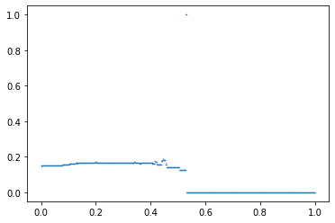
In addition, this index has a plotting method to see the profile estimated.

Spatial Proximity

The Spatial Proximity Index (SP) is given by:

$$ SP = \frac{XP_{xx} + YP_{yy}}{TP_{tt}} $$

where

$$ P_{xx} = \sum_{i_1=1}^{I}\sum_{i_2=1}^{I}\frac{n_{i_1x}n_{i_2x}\zeta_{i_1i_2}}{n_{.x}^2} $$

and

$$ P_{yy} = \sum_{i_1=1}^{I}\sum_{i_2=1}^{I}\frac{n_{i_1y}n_{i_2y}\zeta_{i_1i_2}}{n_{.y}^2} $$

and

$$ P_{tt} = \sum_{i_1=1}^{I}\sum_{i_2=1}^{I}\frac{n_{i_1.}n_{i_2.}\zeta_{i_1i_2}}{n_{..}^2} $$

and

$$ \zeta_{i_1i_2} = exp(-d_{i_1i_2}) $$

$d_{i_1i_2}$ is a pairwise distance measure between area $i_1$ and $i_2$ and $d_{ii}$ is estimated as $d_{ii} = (\alpha a_i)^{\beta}$ where $a_i$ is the area of unit $i$. The default is $\alpha = 0.6$ and $\beta = 0.5$ and for the distance measure, we first extracts the centroid of each unit and calculate the euclidean distance.

The index is fitted below (note you can choose alpha and beta):

Absolute Clustering

The Absolute Clustering Measure (ACL) is given by:

$$ ACL = \frac{\left (\sum_{i_1=1}^{I}\left ( \frac{x_{i_1}}{X} \right )\sum_{i_2=1}^{I}\zeta_{i_1i_2}x_{i_2} \right ) - \left ( \frac{X}{n^2}\sum_{i_1=1}^{I}\sum_{i_2=1}^{I}\zeta_{i_1i_2} \right )}{\left (\sum_{i_1=1}^{I}\left ( \frac{x_{i_1}}{X} \right )\sum_{i_2=1}^{I}\zeta_{i_1i_2}t_{i_2} \right ) - \left ( \frac{X}{n^2}\sum_{i_1=1}^{I}\sum_{i_2=1}^{I}\zeta_{i_1i_2} \right )} $$

The index is fitted below (note you can choose alpha and beta):

Relative Clustering

The Relative Clustering Measure (RCL) is given by:

$$ RCL = \frac{P_{xx}}{P_{yy}} - 1 $$

The index is fitted below (note you can choose alpha and beta):

Distance Decay Isolation

The Distance Decay Isolation (DDxPx) is given by:

$$ DDxPx=\sum_{i_1=1}^{I}\left ( \hat{s}_{i_1x} \right )\left (\sum_{i_2=1}^{I}P_{i_1i_2} \left (\tilde{s}_{i_1x}\right ) \right ) $$

where

$$ P_{i_1i_2} = \frac{\zeta_{i_1i_2}n_{i_2.}}{\sum_{i_2=1}^{I}\zeta_{i_1i_2}n_{i_2.}} $$

such that

$$ \sum_{i_2=1}^{I}P_{i_1i_2} = 1. $$

where $\zeta_{i_1i_2}$ is defined as before. This also could be seen as the probability of contact of members of group $x$ to each other weighted by the inverse of distance.

The index is fitted below (note you can choose alpha and beta):

Distance Decay Exposure

The Distance Decay Exposure (DDxPy) is given by:

$$ DDxPy=\sum_{i_1=1}^{I}\left ( \hat{s}_{i_1x} \right )\left (\sum_{i_2=1}^{I}P_{i_1i_2} \left (\tilde{s}_{i_1y}\right ) \right ) $$

where $P_{i_1i_2}$ is defined as before.

The index is fitted below (note you can choose alpha and beta):

Delta

The Delta (DEL) measure is given by the following equation:

$$ DEL = \frac{1}{2}\sum_{i=1}^{I}\left | \hat{s}_{ij} - \frac{a_i}{A} \right | $$

where $a_i$ is the area of unit $i$ and $A$ is the total area of the given region $A = \sum_{i=1}^{I}a_i$.

The index is fitted below:

Absolute Concentration

The Absolute Concentration Index (ACO) is given by:

$$ \large ACO = 1-\frac{ \sum_{i=1}^{I}\left ( \frac{n_{ij}a_i}{n_{.j}} \right ) - \sum_{i=1}^{n_1}\left ( \frac{n_{i.}a_i}{T_1} \right )}{ \sum_{i=n_2}^{I}\left ( \frac{n_{i.}a_i}{T_2} \right ) - \sum_{i=1}^{n_1}\left ( \frac{n_{i.}a_i}{T_1} \right )} $$

where the units are ordered from smallest to largest in areal size. In this formula, $n_1$ is the rank of the unit where the cumulative total population equal the total minority population, $n_2$ is the rank of the unit where cumulative total population equal equal the total minority population from the largest unit down. In addition,

$$ T_1 = \sum_{i=1}^{n_1}n_{i.} $$

and

$$ T_2 = \sum_{i=n_2}^{n}n_{i.} $$

The index is fitted below:

Relative Concentration

The Relative Concentration Index (RCO) is given by:

$$ \large RCO = \frac{\frac{\sum_{i=1}^{I}\left ( \frac{n_{ix}a_i}{n_{.x}} \right )}{\sum_{i=1}^{I}\left ( \frac{n_{iy}a_i}{n_{.y}} \right )}-1}{\frac{\sum_{i=1}^{n_1}\left ( \frac{n_{i.}a_i}{T_1} \right )}{\sum_{i=n_2}^{I}\left ( \frac{n_{i.}a_i}{T_2} \right )}-1} $$

where $n_1$, $n_2$, $T_1$ and $T_2$ are defined as before.

The index is fitted below:

Absolute Centralization and Relative Centralization

The degree of centralization can be evaluated through the Absolute Centralization Index (ACE) or through the Relative Centralization Index (RCE):

$$ ACE=\left ( \sum_{i=2}^{I}X_{i-1}A_i \right ) - \left ( \sum_{i=2}^{I}X_{i}A_{i-1} \right ) $$

and

$$ RCE=\left ( \sum_{i=2}^{I}X_{i-1}Y_i \right ) - \left ( \sum_{i=2}^{I}X_{i}Y_{i-1} \right ) $$

where $A_i$ is the cumulative area proportion through unit $i$, $X_i$ is the cumulative frequency proportion through unit $i$ of group $x$ and $Y_i$ is the analogous for group $y$. In this measure, the area units are ordered by increasing distances from the central business district, which could be modified with the center argument.

The ACE is fitted below:

The RCE is fitted below:

Spatial Minimum-Maximum Index (SMM)

The Spatial Minimum-Maximum Index (SMM) is the index of O'Sullivan, David, and David WS Wong. "A surface‐based approach to measuring spatial segregation." Geographical Analysis 39.2 (2007): 147-168. Its formula is given by:

$$ SMM = \frac{\sum_{i=1}^{n} max \left ( \hat{s}_{i1}, \hat{s}_{i2} \right ) - \sum_{i=1}^{n} min \left ( \hat{s}_{i1}, \hat{s}_{i2} \right )}{\sum_{i=1}^{n} max \left ( \hat{s}_{i1}, \hat{s}_{i2} \right )} $$

where $\hat{s}_{i1}$ and $\hat{s}_{i2}$ are calculated after performing a spatial smoothing in each population given by w or network (a libpysal Kernel function as default) and the sub-indexes $1$ and $2$ are two mutually exclusive groups (for example, Hispanic and non-Hispanic population). Internally, segregation creates the complementary group of HISP_.