In spatial analysis workflows it is often important and necessary to asses the relationships of neighbouring polygons. libpysal and splot can help you to inspect if two neighbouring polygons share an edge or not.
Content:
- Imports
- Data Preparation
- Plotting
from libpysal.weights.contiguity import Queen
import libpysal
from libpysal import examples
import matplotlib.pyplot as plt
import geopandas as gpd
%matplotlib inline
from splot.libpysal import plot_spatial_weights
Let's first have a look at the dataset with libpysal.examples.explain
examples.explain('rio_grande_do_sul')
Load data into a geopandas geodataframe
gdf = gpd.read_file(examples.get_path('map_RS_BR.shp'))
gdf.head()
weights = Queen.from_dataframe(gdf)
This warning tells us that our dataset contains islands. Islands are polygons that do not share edges and nodes with adjacent polygones. This can for example be the case if polygones are truly not neighbouring, eg. when two land parcels are seperated by a river. However, these islands often stems from human error when digitizing features into polygons.
This unwanted error can be assessed using splot.libpysal plot_spatial_weights functionality:
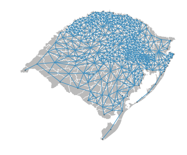
plot_spatial_weights(weights, gdf)
plt.show()
This visualisation depicts the spatial weights network, a network of connections of the centroid of each polygon to the centroid of its neighbour. As we can see, there are many polygons in the south and west of this map, that are not connected to it's neighbors. This stems from digitization errors and needs to be corrected before we can start our statistical analysis.
libpysal offers a tool to correct this error by 'snapping' incorrectly separated neighbours back together:
wnp = libpysal.weights.util.nonplanar_neighbors(weights, gdf)
We can now visualise if the nonplanar_neighbors tool adjusted all errors correctly:
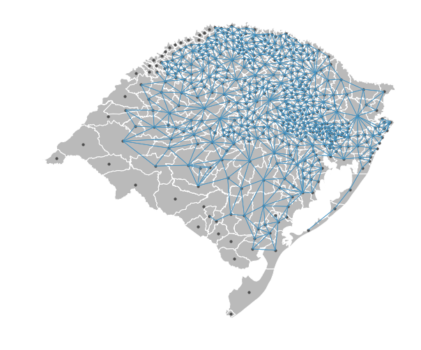
plot_spatial_weights(wnp, gdf)
plt.show()
The visualization shows that all erroneous islands are now stored as neighbors in our new weights object, depicted by the new joins displayed in orange.
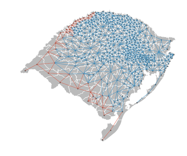
We can now adapt our visualization to show all joins in the same color, by using the nonplanar_edge_kws argument in plot_spatial_weights:
plot_spatial_weights(wnp, gdf, nonplanar_edge_kws=dict(color='#4393c3'))
plt.show()