weights

import sys
import os

sys.path.append(os.path.abspath('..'))
import libpysal

libpysal.examples.available()

['georgia',
 '__pycache__',
 'tests',
 'newHaven',
 'Polygon_Holes',
 'nat',
 'Polygon',
 '10740',
 'berlin',
 'rio_grande_do_sul',
 'sids2',
 'sacramento2',
 'burkitt',
 'arcgis',
 'calemp',
 'stl',
 'virginia',
 'geodanet',
 'desmith',
 'book',
 'nyc_bikes',
 'Line',
 'south',
 'snow_maps',
 'Point',
 'street_net_pts',
 'guerry',
 '__pycache__',
 'baltim',
 'networks',
 'us_income',
 'taz',
 'columbus',
 'tokyo',
 'mexico',
 '__pycache__',
 'chicago',
 'wmat',
 'juvenile',
 'clearwater']

libpysal.examples.explain('mexico')

{'name': 'mexico',
 'description': 'Decennial per capita incomes of Mexican states 1940-2000',
 'explanation': ['* mexico.csv: attribute data. (n=32, k=13)',
  '* mexico.gal: spatial weights in GAL format.',
  '* mexicojoin.shp: Polygon shapefile. (n=32)',
  'Data used in Rey, S.J. and M.L. Sastre Gutierrez. (2010) "Interregional inequality dynamics in Mexico." Spatial Economic Analysis, 5: 277-298.']}

Weights from GeoDataFrames

import geopandas
pth = libpysal.examples.get_path("mexicojoin.shp")
gdf = geopandas.read_file(pth)

from libpysal.weights import Queen, Rook, KNN

%matplotlib inline
import matplotlib.pyplot as plt

ax = gdf.plot()
ax.set_axis_off()

Contiguity Weights

The first set of spatial weights we illustrate use notions of contiguity to define neighboring observations. Rook neighbors are those states that share an edge on their respective borders:

w_rook = Rook.from_dataframe(gdf)

w_rook.n

w_rook.pct_nonzero

12.6953125

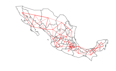
ax = gdf.plot(edgecolor='grey', facecolor='w')
f,ax = w_rook.plot(gdf, ax=ax, 
        edge_kws=dict(color='r', linestyle=':', linewidth=1),
        node_kws=dict(marker=''))
ax.set_axis_off()

gdf.head()

	POLY_ID	AREA	CODE	NAME	PERIMETER	ACRES	HECTARES	PCGDP1940	PCGDP1950	PCGDP1960	...	GR9000	LPCGDP40	LPCGDP50	LPCGDP60	LPCGDP70	LPCGDP80	LPCGDP90	LPCGDP00	TEST	geometry
0	1	7.252751e+10	MX02	Baja California Norte	2040312.385	1.792187e+07	7252751.376	22361.0	20977.0	17865.0	...	0.05	4.35	4.32	4.25	4.40	4.47	4.43	4.48	1.0	(POLYGON ((-113.1397171020508 29.0177764892578...
1	2	7.225988e+10	MX03	Baja California Sur	2912880.772	1.785573e+07	7225987.769	9573.0	16013.0	16707.0	...	0.00	3.98	4.20	4.22	4.39	4.46	4.41	4.42	2.0	(POLYGON ((-111.2061233520508 25.8027763366699...
2	3	2.731957e+10	MX18	Nayarit	1034770.341	6.750785e+06	2731956.859	4836.0	7515.0	7621.0	...	-0.05	3.68	3.88	3.88	4.04	4.13	4.11	4.06	3.0	(POLYGON ((-106.6210784912109 21.5653114318847...
3	4	7.961008e+10	MX14	Jalisco	2324727.436	1.967200e+07	7961008.285	5309.0	8232.0	9953.0	...	0.03	3.73	3.92	4.00	4.21	4.32	4.30	4.33	4.0	POLYGON ((-101.52490234375 21.85663986206055, ...
4	5	5.467030e+09	MX01	Aguascalientes	313895.530	1.350927e+06	546702.985	10384.0	6234.0	8714.0	...	0.13	4.02	3.79	3.94	4.21	4.32	4.32	4.44	5.0	POLYGON ((-101.8461990356445 22.01176071166992...

5 rows × 35 columns

w_rook.neighbors[0] # the first location has two neighbors at locations 1 and 22

[1, 22]

gdf['NAME'][[0, 1,22]]

0     Baja California Norte
1       Baja California Sur
22                   Sonora
Name: NAME, dtype: object

So, Baja California Norte has 2 rook neighbors: Baja California Sur and Sonora.

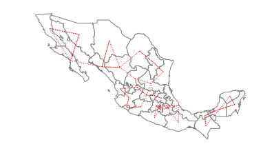
Queen neighbors are based on a more inclusive condition that requires only a shared vertex between two states:

w_queen = Queen.from_dataframe(gdf)

w_queen.n == w_rook.n

True

(w_queen.pct_nonzero > w_rook.pct_nonzero) == (w_queen.n == w_rook.n)

True

ax = gdf.plot(edgecolor='grey', facecolor='w')
f,ax = w_queen.plot(gdf, ax=ax, 
        edge_kws=dict(color='r', linestyle=':', linewidth=1),
        node_kws=dict(marker=''))
ax.set_axis_off()

w_queen.histogram

[(1, 1), (2, 6), (3, 6), (4, 6), (5, 5), (6, 2), (7, 3), (8, 2), (9, 1)]

w_rook.histogram

[(1, 1), (2, 6), (3, 7), (4, 7), (5, 3), (6, 4), (7, 3), (8, 1)]

c9 = [idx for idx,c in w_queen.cardinalities.items() if c==9]

gdf['NAME'][c9]

28    San Luis Potosi
Name: NAME, dtype: object

w_rook.neighbors[28]

[5, 6, 7, 27, 29, 30, 31]

w_queen.neighbors[28]

[3, 5, 6, 7, 24, 27, 29, 30, 31]

import numpy as np
f,ax = plt.subplots(1,2,figsize=(10, 6), subplot_kw=dict(aspect='equal'))
gdf.plot(edgecolor='grey', facecolor='w', ax=ax[0])
w_rook.plot(gdf, ax=ax[0], 
        edge_kws=dict(color='r', linestyle=':', linewidth=1),
        node_kws=dict(marker=''))
ax[0].set_title('Rook')
ax[0].axis(np.asarray([-105.0, -95.0, 21, 26]))

ax[0].axis('off')
gdf.plot(edgecolor='grey', facecolor='w', ax=ax[1])
w_queen.plot(gdf, ax=ax[1], 
        edge_kws=dict(color='r', linestyle=':', linewidth=1),
        node_kws=dict(marker=''))
ax[1].set_title('Queen')
ax[1].axis('off')
ax[1].axis(np.asarray([-105.0, -95.0, 21, 26]))

array([-105.,  -95.,   21.,   26.])

w_knn = KNN.from_dataframe(gdf, k=4)

w_knn.histogram

[(4, 32)]

ax = gdf.plot(edgecolor='grey', facecolor='w')
f,ax = w_knn.plot(gdf, ax=ax, 
        edge_kws=dict(color='r', linestyle=':', linewidth=1),
        node_kws=dict(marker=''))
ax.set_axis_off()

Weights from shapefiles (without geopandas)

pth = libpysal.examples.get_path("mexicojoin.shp")
from libpysal.weights import Queen, Rook, KNN

w_queen = Queen.from_shapefile(pth)

w_rook = Rook.from_shapefile(pth)

w_knn1 = KNN.from_shapefile(pth)

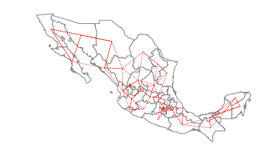
/home/serge/Dropbox/p/pysal/src/subpackages/libpysal/libpysal/weights/weights.py:170: UserWarning: The weights matrix is not fully connected. There are 2 components
  warnings.warn("The weights matrix is not fully connected. There are %d components" % self.n_components)

The warning alerts us to the fact that using a first nearest neighbor criterion to define the neighbors results in a connectivity graph that has more than a single component. In this particular case there are 2 components which can be seen in the following plot:

ax = gdf.plot(edgecolor='grey', facecolor='w')
f,ax = w_knn1.plot(gdf, ax=ax, 
        edge_kws=dict(color='r', linestyle=':', linewidth=1),
        node_kws=dict(marker=''))
ax.set_axis_off()

The two components are separated in the southern part of the country, with the smaller component to the east and the larger component running through the rest of the country to the west. For certain types of spatial analytical methods, it is necessary to have a adjacency structure that consists of a single component. To ensure this for the case of Mexican states, we can increase the number of nearest neighbors to three:

w_knn3 = KNN.from_shapefile(pth,k=3)

ax = gdf.plot(edgecolor='grey', facecolor='w')
f,ax = w_knn3.plot(gdf, ax=ax, 
        edge_kws=dict(color='r', linestyle=':', linewidth=1),
        node_kws=dict(marker=''))
ax.set_axis_off()

Lattice Weights

from libpysal.weights import lat2W

w = lat2W(4,3)

w.n

w.pct_nonzero

23.61111111111111

w.neighbors

{0: [3, 1],
 3: [0, 6, 4],
 1: [0, 4, 2],
 4: [1, 3, 7, 5],
 2: [1, 5],
 5: [2, 4, 8],
 6: [3, 9, 7],
 7: [4, 6, 10, 8],
 8: [5, 7, 11],
 9: [6, 10],
 10: [7, 9, 11],
 11: [8, 10]}

Handling nonplanar geometries

rs = libpysal.examples.get_path('map_RS_BR.shp')

import geopandas as gpd

rs_df = gpd.read_file(rs)
wq = libpysal.weights.Queen.from_dataframe(rs_df)

/home/serge/Dropbox/p/pysal/src/subpackages/libpysal/libpysal/weights/weights.py:168: UserWarning: There are 29 disconnected observations 
  Island ids: 0, 4, 23, 27, 80, 94, 101, 107, 109, 119, 122, 139, 169, 175, 223, 239, 247, 253, 254, 255, 256, 261, 276, 291, 294, 303, 321, 357, 374
  " Island ids: %s" % ', '.join(str(island) for island in self.islands))

len(wq.islands)

wq[0]

{}

wf = libpysal.weights.fuzzy_contiguity(rs_df)

wf.islands

[]

wf[0]

{239: 1.0, 59: 1.0, 152: 1.0, 23: 1.0, 107: 1.0}

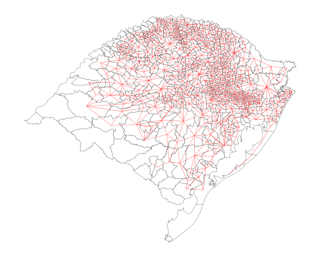
plt.rcParams["figure.figsize"] = (20,15)
ax = rs_df.plot(edgecolor='grey', facecolor='w')
f,ax = wq.plot(rs_df, ax=ax, 
        edge_kws=dict(color='r', linestyle=':', linewidth=1),
        node_kws=dict(marker=''))

ax.set_axis_off()

ax = rs_df.plot(edgecolor='grey', facecolor='w')
f,ax = wf.plot(rs_df, ax=ax, 
        edge_kws=dict(color='r', linestyle=':', linewidth=1),
        node_kws=dict(marker=''))
ax.set_title('Rio Grande do Sul: Nonplanar Weights')
ax.set_axis_off()
plt.savefig('rioGrandeDoSul.png')