network-analysis

If any part of this notebook is used in your research, please cite with the reference found in README.md.

Spatial network analysis

Demonstrating network representation and cluster detection

Author: James D. Gaboardi jgaboardi@gmail.com

This notebook is an advanced walk-through for:

Exploring the attributes of network objects and point patterns
Understanding the difference between a network and its graph-theoretic representation
Performing spatial network analysis

%load_ext watermark
%watermark

2020-01-20T16:01:44-05:00

CPython 3.7.3
IPython 7.10.2

compiler   : Clang 9.0.0 (tags/RELEASE_900/final)
system     : Darwin
release    : 19.2.0
machine    : x86_64
processor  : i386
CPU cores  : 4
interpreter: 64bit

In addtion to the base spaghetti requirements (and their dependecies), this notebook requires installations of:

matplotlib
- $ conda install matplotlib

import spaghetti
import esda
import libpysal
import matplotlib
import matplotlib.pyplot as plt
import numpy
import warnings
try:
    from IPython.display import set_matplotlib_formats
    set_matplotlib_formats("retina")
except ImportError:
    pass
%matplotlib inline
%watermark -w
%watermark -iv

watermark 2.0.2
spaghetti  1.4.0
numpy      1.17.3
libpysal   4.2.0
esda       2.1.1
matplotlib 3.1.2

1. Instantiating a `spaghetti.Network` object

Instantiate the network from a `.shp` file

ntw = spaghetti.Network(in_data=libpysal.examples.get_path("streets.shp"))

2. Allocating observations (snapping points) to a network:

A network is composed of a single topological representation of network elements (arcs and vertices) to which point patterns may be snapped.

# Crimes
ntw.snapobservations(
    libpysal.examples.get_path("crimes.shp"), "crimes", attribute=True
)
# Schools
ntw.snapobservations(
    libpysal.examples.get_path("schools.shp"), "schools", attribute=False
)
ntw.pointpatterns

{'crimes': <spaghetti.network.PointPattern at 0x11c5f0320>,
 'schools': <spaghetti.network.PointPattern at 0x11d553048>}

Attributes for every point pattern

dist_snapped dict keyed by point id with the value as snapped distance from observation to network arc

ntw.pointpatterns["crimes"].dist_snapped[0]

221.5867616973843

dist_to_vertex dict keyed by pointid with the value being a dict in the form
```
 {node: distance to vertex, node: distance to vertex}
```

ntw.pointpatterns["crimes"].dist_to_vertex[0]

{161: 83.70599311338093, 162: 316.8274480625799}

npoints point observations in set

ntw.pointpatterns["crimes"].npoints

obs_to_arc dict keyed by arc with the value being a dict in the form
```
 {pointID:(x-coord, y-coord), pointID:(x-coord, y-coord), ... }
```

ntw.pointpatterns["crimes"].obs_to_arc[(161, 162)]

{0: (727919.2473619275, 875942.4986759046)}

obs_to_vertex list of incident network vertices to snapped observation points

ntw.pointpatterns["crimes"].obs_to_vertex[0]

points geojson like representation of the point pattern. Includes properties if read with attributes=True

ntw.pointpatterns["crimes"].points[0]

{'coordinates': (727913.0000000029, 875720.9999999977), 'properties': [[1, 1]]}

snapped_coordinates dict keyed by pointid with the value being (x-coord, y-coord)

ntw.pointpatterns["crimes"].snapped_coordinates[0]

(727919.2473619275, 875942.4986759046)

Counts per link (arc or edge) are important, but should not be precomputed since we have different representations of the network (spatial and graph currently). (Relatively) Uniform segmentation still needs to be done.

counts = ntw.count_per_link(ntw.pointpatterns["crimes"].obs_to_arc, graph=False)

orig_counts_per_link = sum(list(counts.values())) / float(len(counts.keys()))
orig_counts_per_link

2.682242990654206

3. Network segmentation

Split network arcs into segments of 200 (US feet is this case)

n200 = ntw.split_arcs(200.0)

Calculate observations per link on the segmented network

counts = n200.count_per_link(n200.pointpatterns["crimes"].obs_to_arc, graph=False)
segm_counts_per_link = sum(counts.values()) / float(len(counts.keys()))
segm_counts_per_link

2.0354609929078014

4. Extract `geopandas.GeoDataFrame` objects of the vertices and arcs

# 'full' unsegmented network
vertices_df, arcs_df = spaghetti.element_as_gdf(
    ntw, vertices=ntw.vertex_coords, arcs=ntw.arcs
)
# network segmented at 200-meter increments
vertices200_df, arcs200_df = spaghetti.element_as_gdf(
    n200, vertices=n200.vertex_coords, arcs=n200.arcs
)

5. Visualization demonstration

shapefile derived, unsegmented network with vertices in a larger, blue, semi-opaque form
distance segmented network with small, red, fully opaque vertices

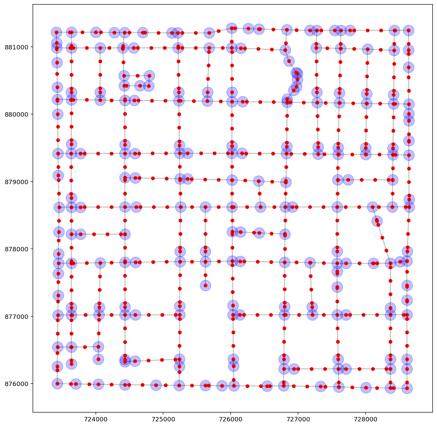
base = arcs_df.plot(color="k", alpha=0.25, figsize=(12, 12))
vertices_df.plot(ax=base, color="b", markersize=300, alpha=0.25)
vertices200_df.plot(ax=base, color="r", markersize=25, alpha=1.0);

6. Spatial Analysis with pysal/esda

6.1 Moran's I using the digitized network

# Compute the counts
counts = ntw.count_per_link(ntw.pointpatterns["crimes"].obs_to_arc, graph=False)

# Binary Adjacency
w = ntw.contiguityweights(graph=False)

# Build the y vector
arcs = w.neighbors.keys()
y = numpy.zeros(len(arcs))

for i, a in enumerate(arcs):
    if a in counts.keys():
        y[i] = counts[a]

# Moran's I
res = esda.moran.Moran(y, w, permutations=99)
print(dir(res))

['EI', 'EI_sim', 'I', 'VI_norm', 'VI_rand', 'VI_sim', '_Moran__calc', '_Moran__moments', '__class__', '__delattr__', '__dict__', '__dir__', '__doc__', '__eq__', '__format__', '__ge__', '__getattribute__', '__gt__', '__hash__', '__init__', '__init_subclass__', '__le__', '__lt__', '__module__', '__ne__', '__new__', '__reduce__', '__reduce_ex__', '__repr__', '__setattr__', '__sizeof__', '__str__', '__subclasshook__', '__weakref__', '_statistic', 'by_col', 'n', 'p_norm', 'p_rand', 'p_sim', 'p_z_sim', 'permutations', 'seI_norm', 'seI_rand', 'seI_sim', 'sim', 'w', 'y', 'z', 'z2ss', 'z_norm', 'z_rand', 'z_sim']

6.2 Moran's I using the graph representation to generate the W

Note that we have to regenerate the counts per arc, since the graph will have less edges.

# Compute the counts
counts = ntw.count_per_link(ntw.pointpatterns["crimes"].obs_to_arc, graph=True)

# Binary Adjacency
w = ntw.contiguityweights(graph=True)

# Build the y vector
edges = w.neighbors.keys()
y = numpy.zeros(len(edges))

for i, e in enumerate(edges):
    if e in counts.keys():
        y[i] = counts[e]

# Moran's I
res = esda.moran.Moran(y, w, permutations=99)

print(dir(res))

['EI', 'EI_sim', 'I', 'VI_norm', 'VI_rand', 'VI_sim', '_Moran__calc', '_Moran__moments', '__class__', '__delattr__', '__dict__', '__dir__', '__doc__', '__eq__', '__format__', '__ge__', '__getattribute__', '__gt__', '__hash__', '__init__', '__init_subclass__', '__le__', '__lt__', '__module__', '__ne__', '__new__', '__reduce__', '__reduce_ex__', '__repr__', '__setattr__', '__sizeof__', '__str__', '__subclasshook__', '__weakref__', '_statistic', 'by_col', 'n', 'p_norm', 'p_rand', 'p_sim', 'p_z_sim', 'permutations', 'seI_norm', 'seI_rand', 'seI_sim', 'sim', 'w', 'y', 'z', 'z2ss', 'z_norm', 'z_rand', 'z_sim']

6.3 Moran's I using the segmented network and intensities instead of counts

# Compute the counts
counts = n200.count_per_link(n200.pointpatterns["crimes"].obs_to_arc, graph=False)

# Binary Adjacency
w = n200.contiguityweights(graph=False)

# Build the y vector and convert from raw counts to intensities
arcs = w.neighbors.keys()
y = numpy.zeros(len(n200.arcs))

for i, a in enumerate(arcs):
    if a in counts.keys():
        length = n200.arc_lengths[a]
        y[i] = float(counts[a]) / float(length)

# Moran's I
res = esda.moran.Moran(y, w, permutations=99)

print(dir(res))

['EI', 'EI_sim', 'I', 'VI_norm', 'VI_rand', 'VI_sim', '_Moran__calc', '_Moran__moments', '__class__', '__delattr__', '__dict__', '__dir__', '__doc__', '__eq__', '__format__', '__ge__', '__getattribute__', '__gt__', '__hash__', '__init__', '__init_subclass__', '__le__', '__lt__', '__module__', '__ne__', '__new__', '__reduce__', '__reduce_ex__', '__repr__', '__setattr__', '__sizeof__', '__str__', '__subclasshook__', '__weakref__', '_statistic', 'by_col', 'n', 'p_norm', 'p_rand', 'p_sim', 'p_z_sim', 'permutations', 'seI_norm', 'seI_rand', 'seI_sim', 'sim', 'w', 'y', 'z', 'z2ss', 'z_norm', 'z_rand', 'z_sim']

7. Simulate a point pattern on the network

Need to supply a count of the number of points and a distirbution (default is uniform). Generally, this will not be called by the user, since the simulation will be used for Monte Carlo permutation.

npts = ntw.pointpatterns["crimes"].npoints
sim = ntw.simulate_observations(npts)
print(dir(sim))

['__class__', '__delattr__', '__dict__', '__dir__', '__doc__', '__eq__', '__format__', '__ge__', '__getattribute__', '__gt__', '__hash__', '__init__', '__init_subclass__', '__le__', '__lt__', '__module__', '__ne__', '__new__', '__reduce__', '__reduce_ex__', '__repr__', '__setattr__', '__sizeof__', '__str__', '__subclasshook__', '__weakref__', 'dist_to_vertex', 'npoints', 'obs_to_arc', 'obs_to_vertex', 'points', 'snapped_coordinates']

8. Network-constrained observation cluster testing

F-function

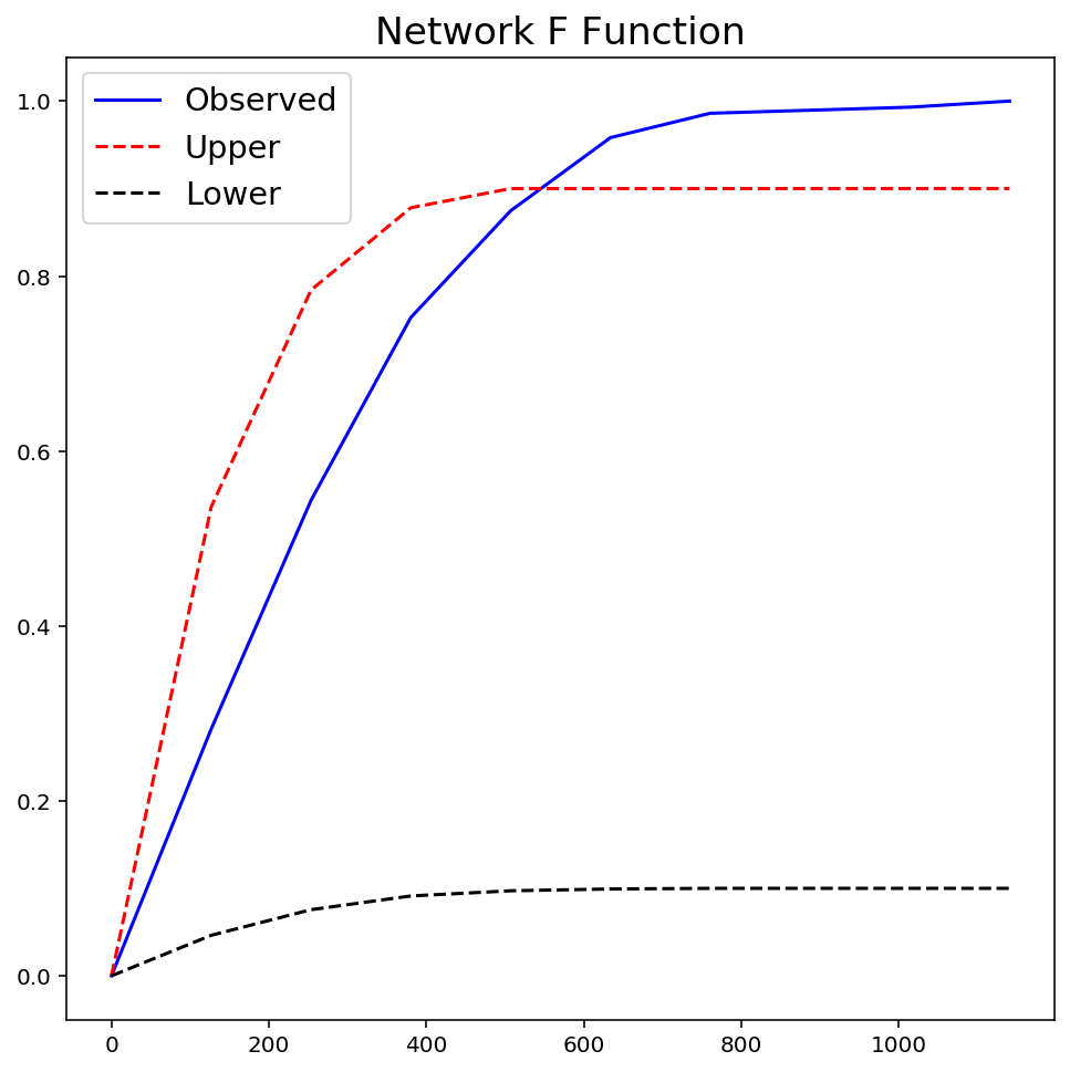
fres = ntw.NetworkF(ntw.pointpatterns["crimes"], permutations=99)

plt.figure(figsize=(8, 8))
plt.plot(fres.xaxis, fres.observed, "b-", linewidth=1.5, label="Observed")
plt.plot(fres.xaxis, fres.upperenvelope, "r--", label="Upper")
plt.plot(fres.xaxis, fres.lowerenvelope, "k--", label="Lower")
plt.legend(loc="best", fontsize="x-large")
plt.title("Network F Function", fontsize="xx-large")
plt.show()

G-function

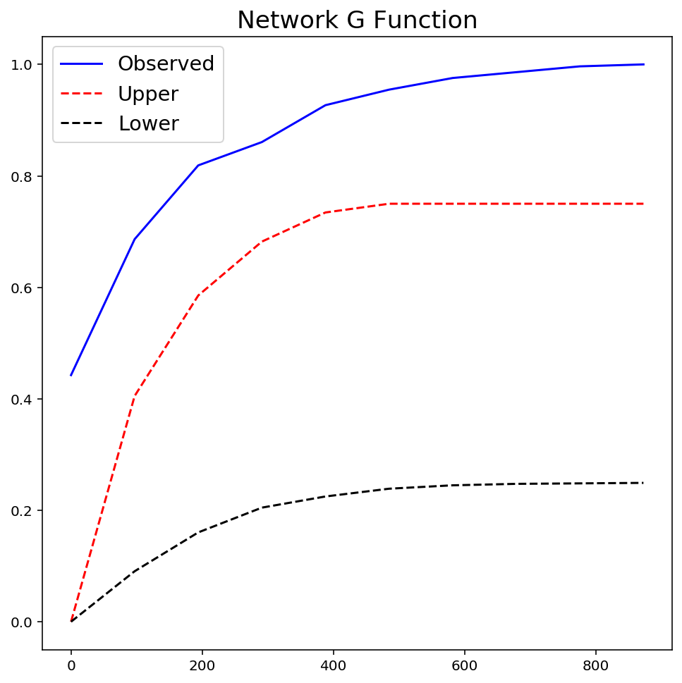
gres = ntw.NetworkG(ntw.pointpatterns["crimes"], permutations=99)

plt.figure(figsize=(8, 8))
plt.plot(gres.xaxis, gres.observed, "b-", linewidth=1.5, label="Observed")
plt.plot(gres.xaxis, gres.upperenvelope, "r--", label="Upper")
plt.plot(gres.xaxis, gres.lowerenvelope, "k--", label="Lower")
plt.legend(loc="best", fontsize="x-large")
plt.title("Network G Function", fontsize="xx-large")
plt.show()

K-function

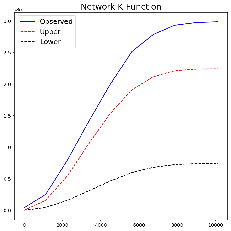
warnings.filterwarnings("ignore", message="invalid value encountered")
kres = ntw.NetworkK(ntw.pointpatterns["crimes"], permutations=99)

plt.figure(figsize=(8, 8))
plt.plot(kres.xaxis, kres.observed, "b-", linewidth=1.5, label="Observed")
plt.plot(kres.xaxis, kres.upperenvelope, "r--", label="Upper")
plt.plot(kres.xaxis, kres.lowerenvelope, "k--", label="Lower")
plt.legend(loc="best", fontsize="x-large")
plt.title("Network K Function", fontsize="xx-large")
plt.show()