This page was generated from notebooks/skater.ipynb. Interactive online version:

SKATER

Spatial ‘K’luster Analysis by Tree Edge Removal: Clustering Airbnb Spots in Chicago

Authors: Xin Feng, James Gaboardi

---

The tutorial is broken out as follows:

1. An explanation of the SKATER algorithm

2. Supporting data: Airbnb Spots in Chicago

3. Understanding parameters

4. Regionalization

5. Exploring parameters

%config InlineBackend.figure_format = "retina"
%load_ext watermark
%watermark

Last updated: 2023-12-10T14:11:06.498766-05:00

Python implementation: CPython
Python version       : 3.12.0
IPython version      : 8.18.0

Compiler    : Clang 15.0.7
OS          : Darwin
Release     : 23.1.0
Machine     : x86_64
Processor   : i386
CPU cores   : 8
Architecture: 64bit

import geopandas
import libpysal
import matplotlib.pyplot as plt
import numpy
import pandas
import shapely
from sklearn.metrics import pairwise as skm
import spopt
import warnings

%matplotlib inline
%watermark -w
%watermark -iv

Watermark: 2.4.3

matplotlib: 3.8.2
numpy     : 1.26.2
pandas    : 2.1.3
libpysal  : 4.9.2
geopandas : 0.14.1
shapely   : 2.0.2
sklearn   : 1.3.2
spopt     : 0.5.1.dev53+g5cadae7

1. An explanation of the SKATER algorithm

SKATER (Assunção et al. 2006) is a constrained spatial regionalization algorithm based on spanning tree pruning. The number of edges is pre-specified to be cut in a continuous tree to group spatial units into contiguous regions.

The first step of SKATER is to create a connectivity graph that captures the neighbourhood relationship between the spatial objects. The cost of each edge in the graph is inversely proportional to the similarity between the regions it joins. The neighbourhood is structured by a minimum spanning tree (MST), which is a connected tree with no circuits. The next step is to partition the MST by successive removal of edges that link dissimilar regions. The final result is the division of the spatial objects into connected regions that have maximum internal homogeneity.

• RM Assunção, MC Neves, G Câmara, and C da Costa Freitas. Efficient regionalization techniques for socio-economic geographical units using minimum spanning trees. International Journal of Geographical Information Science, 20(7):797–811, 2006. doi: 10.1080/13658810600665111.

See also Dmitry Shkolnik’s tutorial of the SKATER algorithm implemented in Roger Bivand’s R package, spdep.

---

2. Supporting data: Airbnb Spots in Chicago

To illustrate Skater we utilize data on Airbnb spots in Chicago, which can be downloaded from libpysal.examples. The data is broken down into 77 communites in Chicago, Illinois from 2015, where a number of attributes are listed for each community.

libpysal.examples.load_example("AirBnB")

<libpysal.examples.base.Example at 0x15a3d8dd0>

chicago = geopandas.read_file(libpysal.examples.get_path("airbnb_Chicago 2015.shp"))
chicago.shape

(77, 21)

chicago.loc[0]

community                                               DOUGLAS
shape_area                                        46004621.1581
shape_len                                         31027.0545098
AREAID                                                       35
response_r                                            98.771429
accept_r                                              94.514286
rev_rating                                            87.777778
price_pp                                              78.157895
room_type                                              1.789474
num_spots                                                    38
poverty                                                    29.6
crowded                                                     1.8
dependency                                                 30.7
without_hs                                                 14.3
unemployed                                                 18.2
income_pc                                                 23791
harship_in                                                   47
num_crimes                                                 5013
num_theft                                                  1241
population                                                18238
geometry      POLYGON ((-87.60914087617012 41.84469250346108...
Name: 0, dtype: object

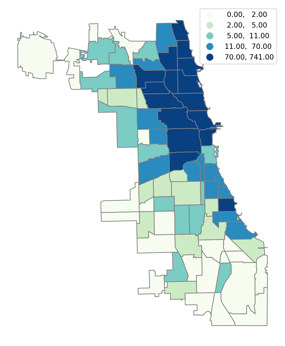
We can visualize the data by plotting the number of Airbnb spots in each community in the sample, using a quintile classification:

chicago.plot(
    figsize=(7, 14),
    column="num_spots",
    scheme="Quantiles",
    cmap="GnBu",
    edgecolor="grey",
    legend=True
).axis("off");

---

3. Understanding parameters

With Skater, we can cluster these 77 communities into 5 regions such that each region consists of at least 5 communities. The homogeneity of the number of Airbnb spots per community within the regions is maximized.

We first define the variable that will be used to measure regional homogeneity, which is the number of Airbnb spots in this case.

attrs_name = ["num_spots"]

Next, we specify a number of other parameters that will serve as input to the skater model, including the spatial weights (to describe the relationship between the spatial objects), the number of regions to include in the solution, the minimal threshold of spatial objects in each region, etc.

A spatial weights object describes the spatial connectivity of the spatial objects:

w = libpysal.weights.Queen.from_dataframe(chicago, use_index=False)

The number of contiguous regions that we would like to group spatial units into:

n_clusters = 5

The minimum number of spatial objects in each region：

floor = 5

trace is a bool denoting whether to store intermediate labelings as the tree gets pruned.

trace = False

The islands keyword argument describes what is to be done with islands. It can be set to either 'ignore', which will treat each island as its own region when solving for n_clusters regions, or 'increase', which will consider each island as its own region and add to n_clusters regions.

islands = "increase"

We can also specify some keywords as input to the spanning forest algorithm, including:

• dissimilarity

  • A callable distance metric, with the default as sklearn.metrics.pairwise.manhattan_distances.

• affinity

  • A callable affinity metric between 0 and 1, which is inverted to provide a dissimilarity metric. No metric is provided as a default (None). If affinity is desired, dissimilarity must explicitly be set to None.

• reduction

  • The reduction applied over all clusters to provide the map score, with the default as numpy.sum().

• center

  • The method for computing the center of each region in attribute space with the default as numpy.mean().

• verbose

  • A flag for how much output to provide to the user in terms of print statements and progress bars. Set to 1 for minimal output and 2 for full output. The default is False, which provides no output.

See spopt.region.skater.SpanningForest for documentation.

spanning_forest_kwds = dict(
    dissimilarity=skm.manhattan_distances,
    affinity=None,
    reduction=numpy.sum,
    center=numpy.mean,
    verbose=2
)

4. Regionalization

The model can then be instantiated and solved:

model = spopt.region.Skater(
    chicago,
    w,
    attrs_name,
    n_clusters=n_clusters,
    floor=floor,
    trace=trace,
    islands=islands,
    spanning_forest_kwds=spanning_forest_kwds
)
model.solve()

Computing Affinity Kernel took 0.00s
Computing initial MST took 0.00s
Computing connected components took 0.00s.

making cut deletion(in_node=45, out_node=67, score=3445.5)...

making cut deletion(in_node=13, out_node=15, score=2574.6813186813188)...

making cut deletion(in_node=2, out_node=34, score=2146.556998556998)...

making cut deletion(in_node=3, out_node=34, score=2025.520634920635)...

Region labels can then be added to the GeoDataFrame from the model object and used for plotting.

chicago["demo_regions"] = model.labels_

chicago.plot(
    figsize=(7, 14), column="demo_regions", categorical=True, edgecolor="w"
).axis("off");

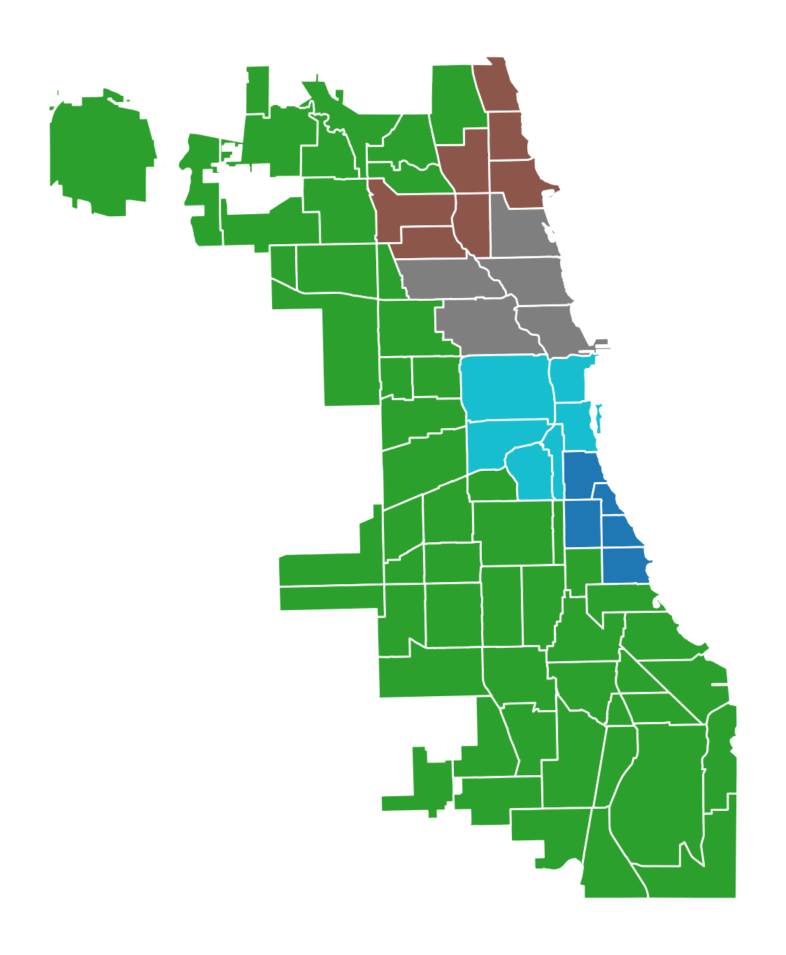
The model solution results in five regions, two of which have five communities, one with six, one with seven, and one with fifty-four.

chicago["count"] = 1
chicago[["demo_regions", "count"]].groupby(by="demo_regions").count()

	count
demo_regions
0	5
1	54
2	7
3	5
4	6

---

5. Exploring parameters

There are myriad parameter combinations that can be passed in for regionalizing with Skater. Here we will explore two combinations of parameters.

• Increasing n_clusters while holding all other parameters constant

• Increasing floor while holding all other parameters constant

• Clustering on multiple variables

Increasing n_clusters

Let’s see how regionalization results differ when increasing n_clusters from 2 to 10 by increments of 2.

n_clusters_range = [2, 4, 6, 8, 10]
n_clusters_range

[2, 4, 6, 8, 10]

For each regionalization run we will hold the other parameters constant.

floor, trace, islands = 5, False, "increase"
spanning_forest_kwds = dict(
    dissimilarity=skm.manhattan_distances,
    affinity=None,
    reduction=numpy.sum,
    center=numpy.mean,
    verbose=False
)

Solve.

for ncluster in n_clusters_range:
    model = spopt.region.Skater(
        chicago,
        w,
        attrs_name,
        n_clusters=ncluster,
        floor=floor,
        trace=trace,
        islands=islands,
        spanning_forest_kwds=spanning_forest_kwds
    )
    model.solve()
    chicago[f"clusters_{ncluster}"] = model.labels_

Plot results.

f, axarr = plt.subplots(1, len(n_clusters_range), figsize=(9, 7.5))
for ix, clust in enumerate(n_clusters_range):
    label = f"clusters_{clust}"
    chicago.plot(column=label, ax=axarr[ix], cmap="tab20")
    axarr[ix].set_title(label)
    axarr[ix].set_axis_off()
plt.subplots_adjust(wspace=1, hspace=0.5)
plt.tight_layout()

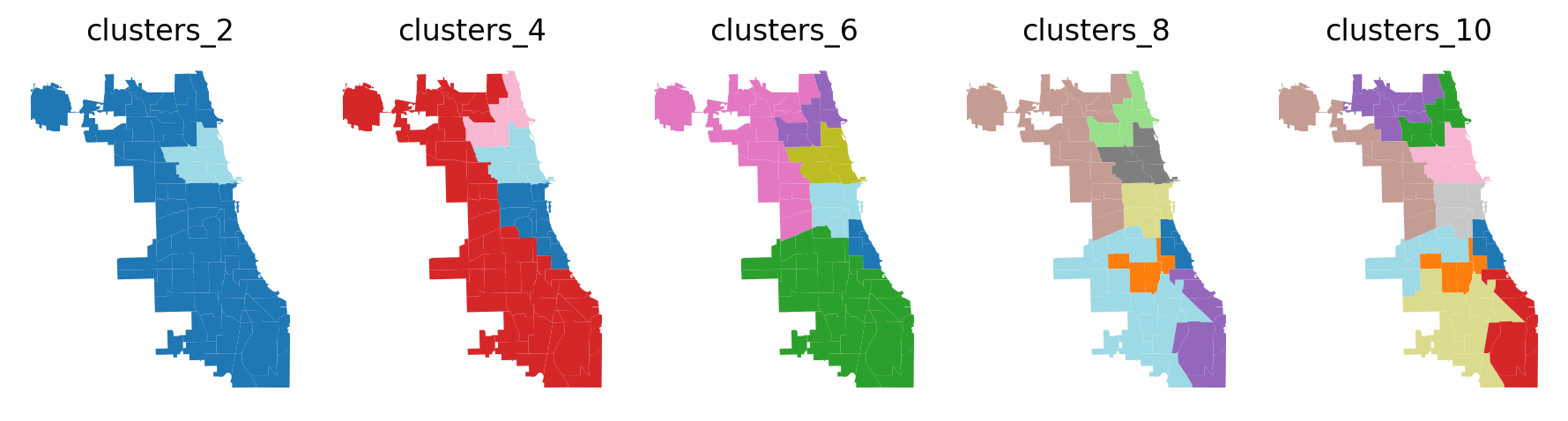
Above we can see that regions become more dispersed and boundaries become more consistent as the number of desired clusters increases. Also, we can investigate the count of communities and the number of AirBnB spots per region, as shown below.

attr1, attr2 = "count", "num_spots"
df = pandas.DataFrame(
    columns=pandas.MultiIndex.from_product(
        [[f"clusters_{i}" for i in n_clusters_range], [attr1, attr2]]
    ),
    index=range(10)
)
df.index.name = "region_id"
for i in n_clusters_range:
    col = f"clusters_{i}"
    df[col, attr1] = chicago[[col, attr1]].groupby(by=col).count()[attr1]
    df[col, attr2] = chicago[[col, attr2]].groupby(by=col).sum()[attr2]
df.fillna(0).astype(int).astype(str).replace("0", "-")

	clusters_2		clusters_4		clusters_6		clusters_8		clusters_10
	count	num_spots	count	num_spots	count	num_spots	count	num_spots	count	num_spots
region_id
0	72	2321	11	963	5	236	5	236	5	236
1	5	2705	54	429	35	143	5	38	5	38
2	-	-	7	929	7	929	7	929	7	929
3	-	-	5	2705	19	286	7	60	7	60
4	-	-	-	-	5	2705	19	286	8	147
5	-	-	-	-	6	727	5	2705	11	139
6	-	-	-	-	-	-	6	727	5	2705
7	-	-	-	-	-	-	23	45	6	727
8	-	-	-	-	-	-	-	-	15	25
9	-	-	-	-	-	-	-	-	8	20

Increasing floor

Next we’ll increase floor from 3 to 15 by increments of 3.

floor_range = [3, 6, 9, 12, 15]
floor_range

[3, 6, 9, 12, 15]

For each regionalization run we will hold the other parameters constant.

n_clusters, trace, islands = 3, True, "increase"
spanning_forest_kwds = dict(
    dissimilarity=None,
    affinity=skm.euclidean_distances,
    reduction=numpy.sum,
    center=numpy.std,
    verbose=False
)

Solve.

for floor in floor_range:
    model = spopt.region.Skater(
        chicago,
        w,
        attrs_name,
        n_clusters=n_clusters,
        floor=floor,
        trace=trace,
        islands=islands,
        spanning_forest_kwds=spanning_forest_kwds
    )
    with warnings.catch_warnings():
        # due to `affinity`
        warnings.filterwarnings(
            "ignore",
            category=RuntimeWarning,
            message="divide by zero encountered in log",
        )
        model.solve()
    chicago[f"floor_{floor}"] = model.labels_

Plot results.

f, axarr = plt.subplots(1, len(floor_range), figsize=(9, 7.5))
for ix, floor in enumerate(floor_range):
    label = f"floor_{floor}"
    chicago.plot(column=label, ax=axarr[ix], cmap="tab20")
    axarr[ix].set_title(label)
    axarr[ix].set_axis_off()
plt.subplots_adjust(wspace=1, hspace=0.5)
plt.tight_layout()

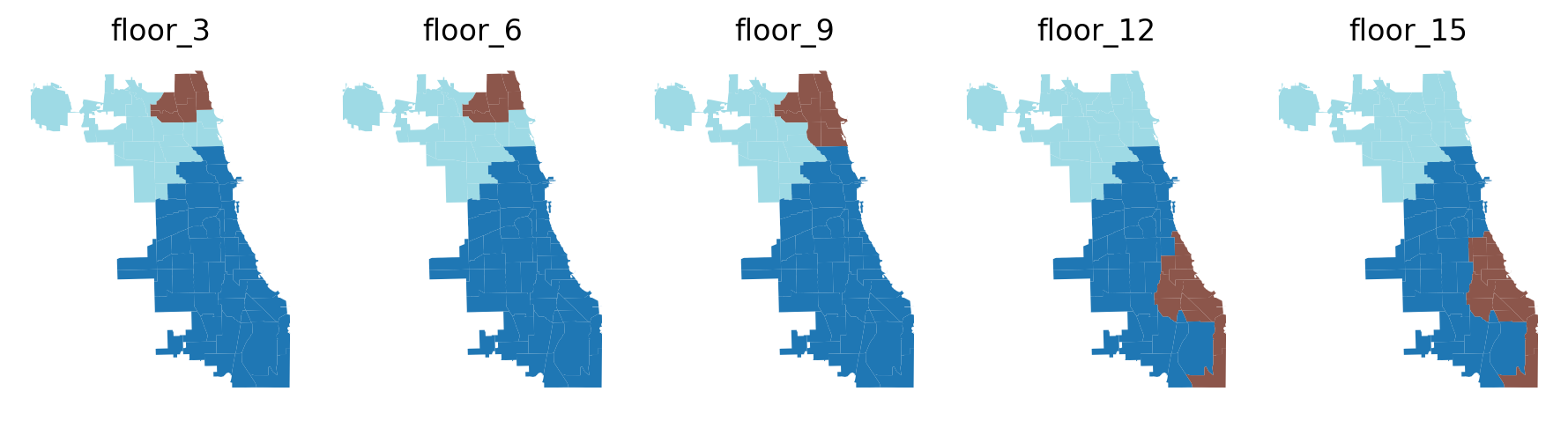
Above we can see an interesting pattern. Boundaries are fixed when stipulating a minimum of 3 and 6 communities per region then the smallest region increases by 3 communities when stipulating floor==9. However, as the minimum number of communities is increased to 12 and 15 the location, shape, and rank of the 3 desired regions vary greatly. See the count of communities and the number of AirBnB spots per region below.

attr1, attr2 = "count", "num_spots"
df = pandas.DataFrame(
    columns=pandas.MultiIndex.from_product(
        [[f"floor_{i}" for i in floor_range], [attr1, attr2]]
    ),
    index=range(3)
)
df.index.name = "region_id"
for i in floor_range:
    col = f"floor_{i}"
    df[col, attr1] = chicago[[col, attr1]].groupby(by=col).count()[attr1]
    df[col, attr2] = chicago[[col, attr2]].groupby(by=col).sum()[attr2]
df

	floor_3		floor_6		floor_9		floor_12		floor_15
	count	num_spots	count	num_spots	count	num_spots	count	num_spots	count	num_spots
region_id
0	52	2867	52	2867	52	2867	39	2637	37	2601
1	6	504	6	504	9	1440	13	230	15	266
2	19	1655	19	1655	16	719	25	2159	25	2159

Clustering on more than one variable

First, let’s isolate some of the variables in the dataset that are characterisitc of social vulnerability.

attrs_name = [
    "poverty",
    "crowded",
    "without_hs",
    "unemployed",
    "harship_in",
    "num_crimes",
    "num_theft"
]

Not all values are available in all communities for each variable, so we’ll set those to 0.

for i in attrs_name:
    chicago[i] = chicago[i].fillna(0)

Now we’ll see how regionalization results differ when increasing n_clusters from 3 to 7 by increments of 1 while considering the 7 social vulnerability variables.

n_clusters_range = [3, 4, 5, 6, 7]
n_clusters_range

[3, 4, 5, 6, 7]

For each regionalization run we will hold the other parameters constant.

floor, trace, islands = 8, True, "increase"
spanning_forest_kwds = dict(
    dissimilarity=skm.manhattan_distances,
    affinity=None,
    reduction=numpy.sum,
    center=numpy.mean,
    verbose=False
)

Solve.

for ncluster in n_clusters_range:
    model = spopt.region.Skater(
        chicago,
        w,
        attrs_name,
        n_clusters=ncluster,
        floor=floor,
        trace=trace,
        islands=islands,
        spanning_forest_kwds=spanning_forest_kwds
    )
    model.solve()
    chicago[f"clusters_{ncluster}"] = model.labels_

Plot results.

f, axarr = plt.subplots(1, len(n_clusters_range), figsize=(9, 7.5))
for ix, clust in enumerate(n_clusters_range):
    label = f"clusters_{clust}"
    chicago.plot(column=label, ax=axarr[ix], cmap="tab20")
    axarr[ix].set_title(label)
    axarr[ix].set_axis_off()
plt.subplots_adjust(wspace=1, hspace=0.5)
plt.tight_layout()

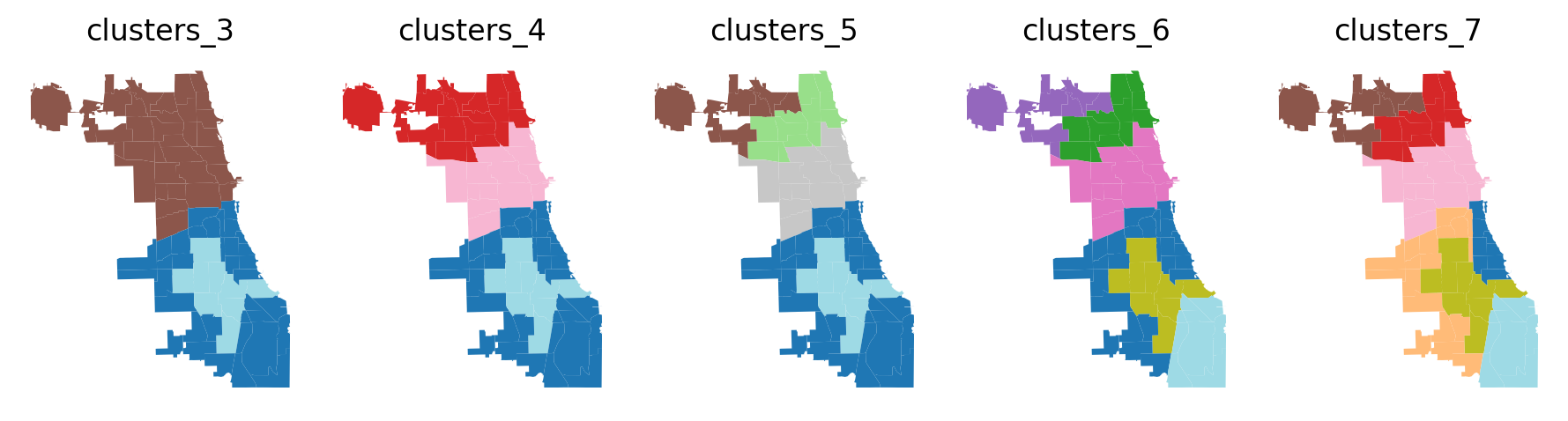
When considering multiple related variables certain cores regions are present in all solutions.

---