This page was generated from notebooks/azp.ipynb.
Interactive online version:
![]()
Automatic Zoning Procedure (AZP) algorithm
Authors: Xin Feng, James Gaboardi
AZP can work with different types of objective functions, which are very sensitive to aggregating data from a large number of zones into a pre-designated smaller number of regions. AZP was originally formulated in Openshaw, 1977 and then extended in Openshaw, S. and Rao, L. (1995).
[1]:
%config InlineBackend.figure_format = "retina"
%load_ext watermark
%watermark
Last updated: 2025-04-07T13:53:10.559404-04:00

Python implementation: CPython
Python version       : 3.12.9
IPython version      : 9.0.2

Compiler    : Clang 18.1.8
OS          : Darwin
Release     : 24.4.0
Machine     : arm64
Processor   : arm
CPU cores   : 8
Architecture: 64bit
[2]:
import warnings

import geopandas
import libpysal

import spopt
from spopt.region import AZP

%matplotlib inline
%watermark -w
%watermark -iv
Watermark: 2.5.0

spopt    : 0.6.2.dev3+g13ca45e
geopandas: 1.0.1
libpysal : 4.12.1
Mexican State Regional Income Clustering
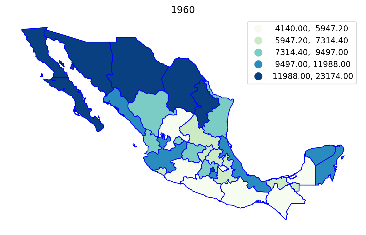
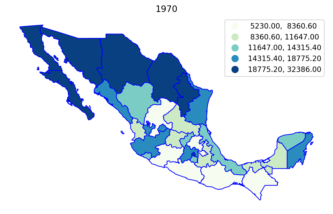
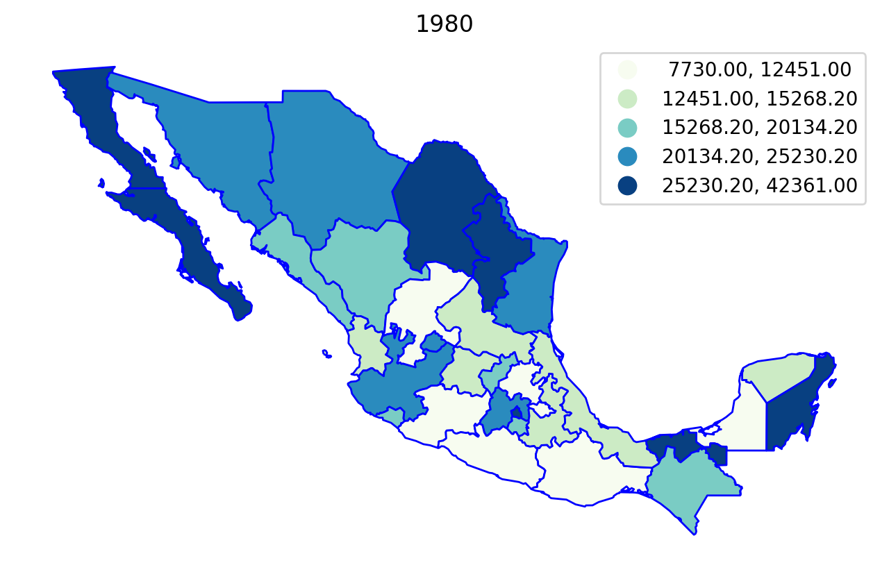
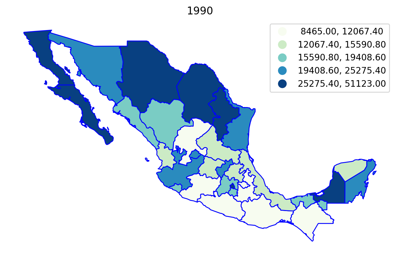
To illustrate azp we utilize data on regional incomes for Mexican states over the period 1940-2000, originally used in Rey and Sastré-Gutiérrez (2010).
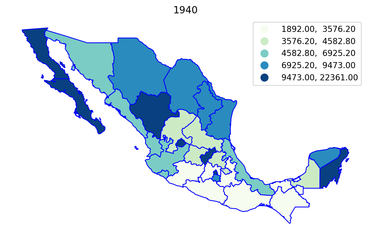
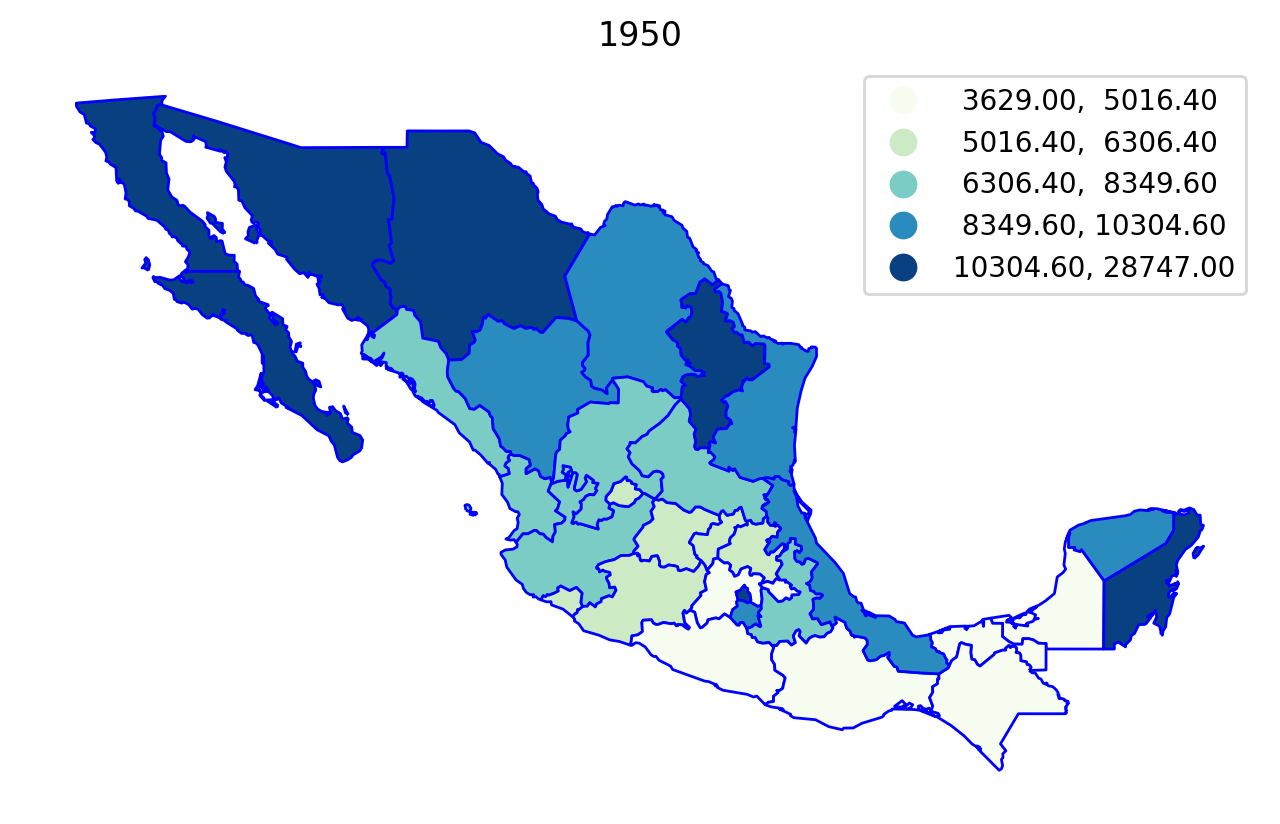
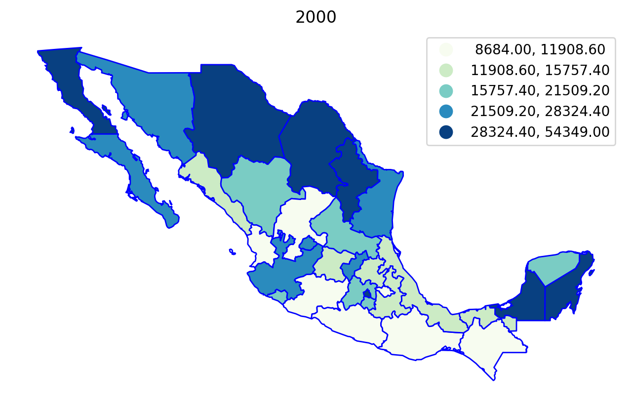
We can first explore the data by plotting the per capital gross regional domestic product (in constant USD 2000 dollars) for each year in the sample, using a quintile classification:
[3]:
pth = libpysal.examples.get_path("mexicojoin.shp")
mexico = geopandas.read_file(pth)
[4]:
for year in range(1940, 2010, 10):
    base = mexico.plot(
        figsize=(8, 5),
        column=f"PCGDP{year}",
        scheme="Quantiles",
        cmap="GnBu",
        edgecolor="b",
        legend=True,
    )
    base.axis("off")
    base.set_title(str(year))
Regionalization
First, we specify a number of parameters that will serve as input to the azp model.
The variables in the dataframe that will be used to measure regional dissimilarity:
[5]:
attrs_name = [f"PCGDP{year}" for year in range(1950, 2010, 10)]
attrs_name
[5]:
['PCGDP1950', 'PCGDP1960', 'PCGDP1970', 'PCGDP1980', 'PCGDP1990', 'PCGDP2000']
A spatial weights object expresses the spatial connectivity of the zones:
[6]:
with warnings.catch_warnings(record=True):
    w = libpysal.weights.Queen.from_dataframe(mexico)
The number of regions that we would like to aggregate these zones into:
[7]:
n_clusters = 5
There are four optional parameters. In this example, we only use the default settings, you can define them as needed.
allow_move_strategy: For a different behavior for allowing moves, an AllowMoveStrategy instance can be passed as argument.
class: AllowMoveStrategy or None, default: None
random_state: Random seed.
None, int, str, bytes, or bytearray, default: None
initial_labels: One-dimensional array of labels at the beginning of the algorithm.
class: numpy.ndarray or None, default: None
If None, then a random initial clustering will be generated.
objective_func: the objective function to use.
class: spopt.region.objective_function.ObjectiveFunction, default: ObjectiveFunctionPairwise()
The model can then be solved:
[8]:
model = AZP(mexico, w, attrs_name, n_clusters)
model.solve()
[9]:
mexico["azp_new"] = model.labels_
[10]:
mexico["number"] = 1
mexico[["azp_new", "number"]].groupby(by="azp_new").count()
[10]:
| number | |
|---|---|
| azp_new | |
| 0.0 | 6 |
| 1.0 | 4 |
| 2.0 | 4 |
| 3.0 | 9 |
| 4.0 | 9 |
[11]:
mexico.plot(figsize=(8, 5), column="azp_new", categorical=True, ec="w").axis("off");
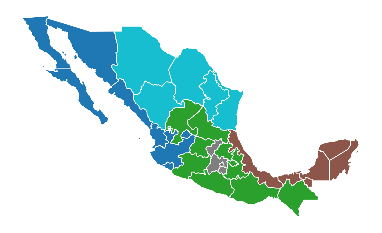
The model solution results in five regions, two of which have five states, one with four, one with eight, and one with ten states.
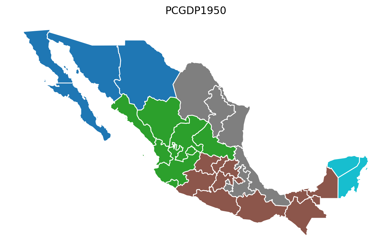
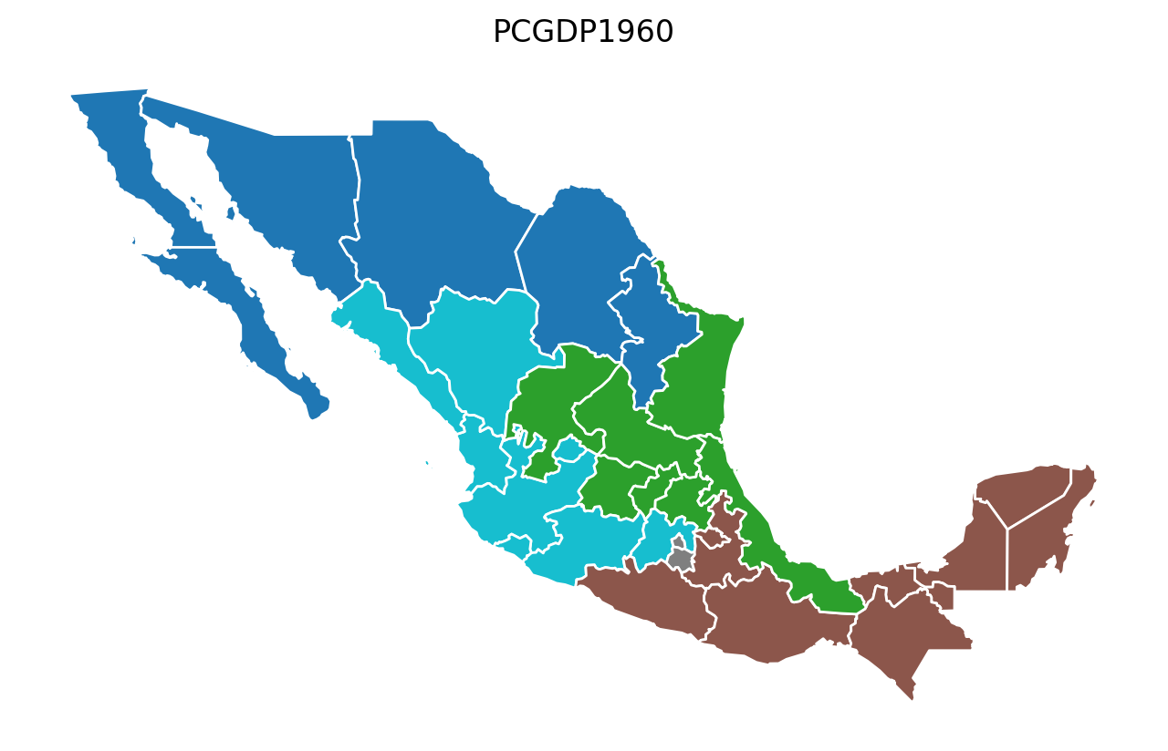
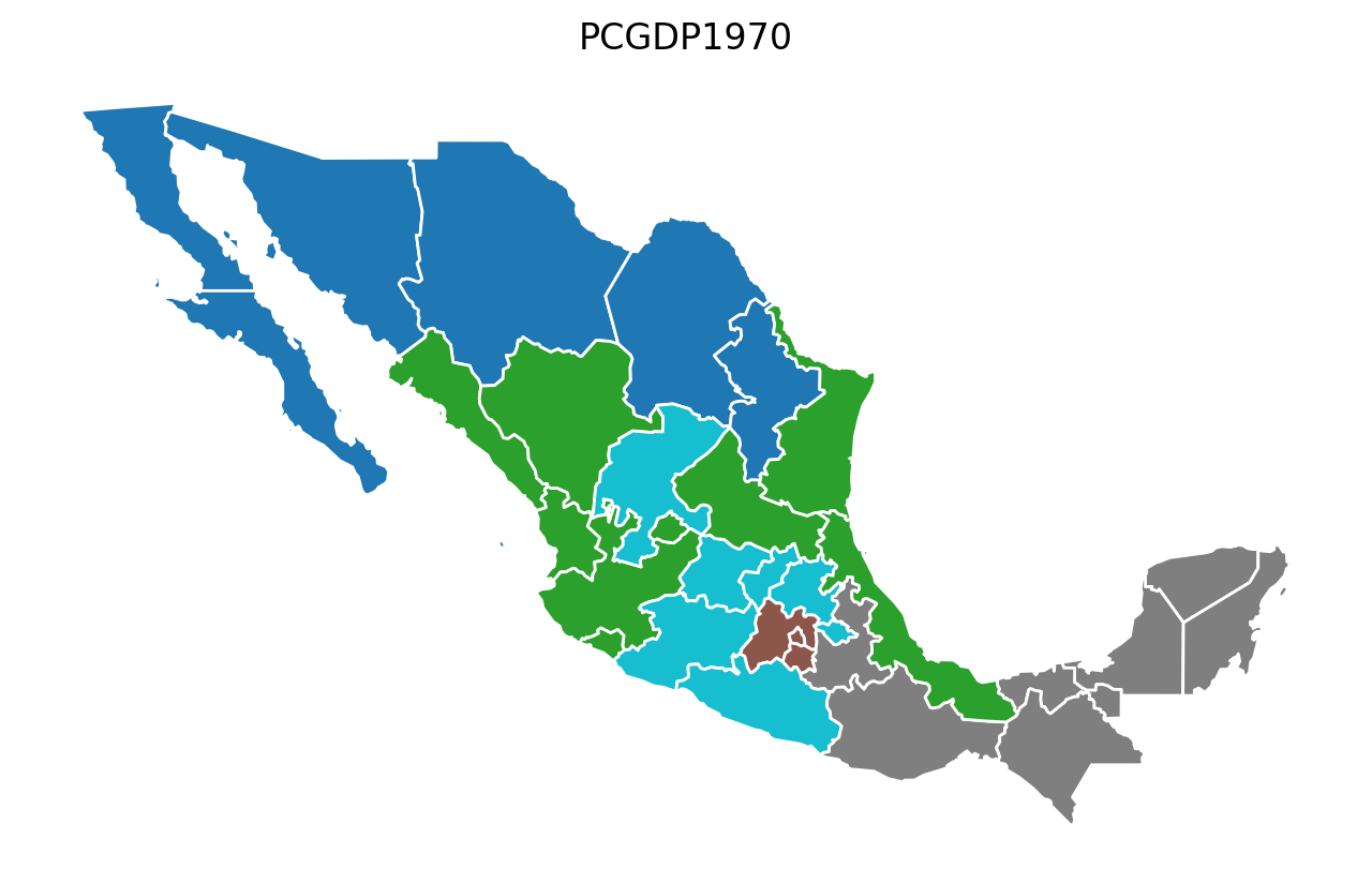
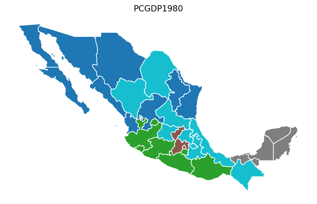
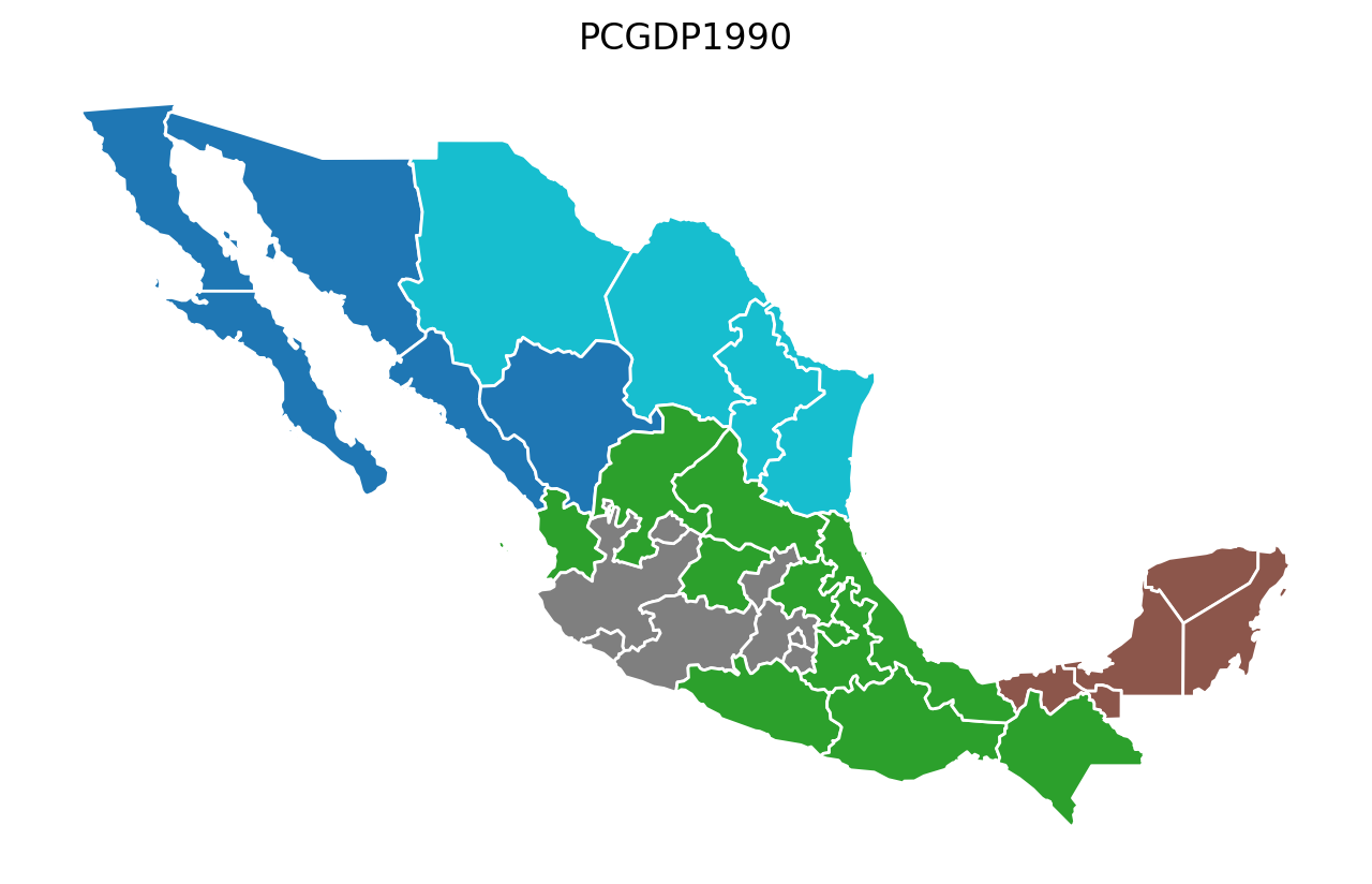
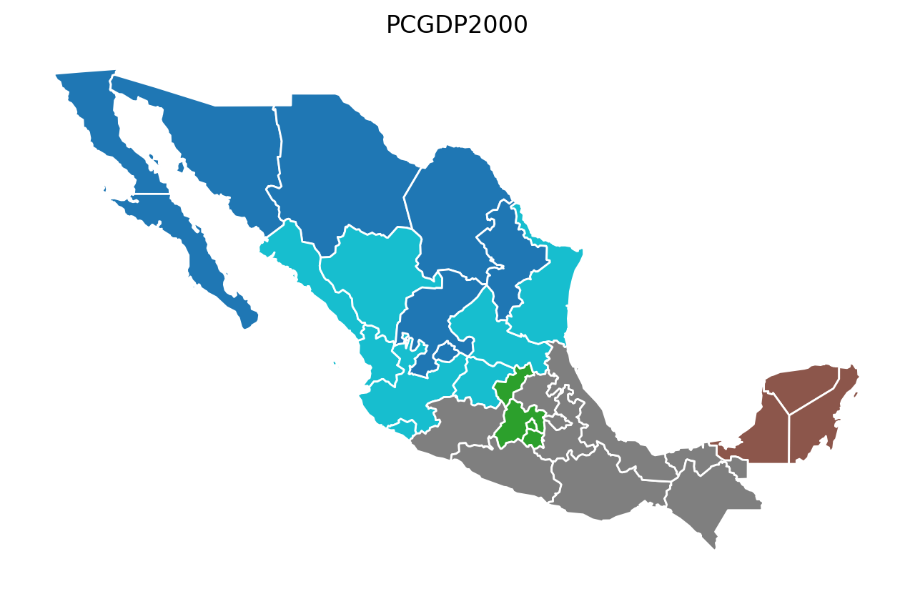
Year-by-Year Regionalization (n_clusters = 5 regions)
[12]:
for year in attrs_name:
    model = AZP(mexico, w, year, 5)
    model.solve()
    lab = year + "labels_"
    mexico[lab] = model.labels_
    base = mexico.plot(figsize=(8, 5), column=lab, categorical=True, edgecolor="w")
    base.axis("off")
    base.set_title(year)