This page was generated from notebooks/reg-k-means.ipynb.
Interactive online version:
![]()
Regional-k-means
Authors: Sergio Rey, Xin Feng, James Gaboardi
Regional-k-means is K-means with the constraint that each cluster forms a spatially connected component. The algorithm is developed by Sergio Rey. This tutorial goes through the following:
a small synthetic example (10x10 lattice)
a large synthetic example (50x50 lattice)
an empirical example (Rio Grande do Sul, Brasil)
[1]:
%config InlineBackend.figure_format = "retina"
%load_ext watermark
%watermark
Last updated: 2025-04-07T15:08:14.668476-04:00

Python implementation: CPython
Python version       : 3.12.9
IPython version      : 9.0.2

Compiler    : Clang 18.1.8
OS          : Darwin
Release     : 24.4.0
Machine     : arm64
Processor   : arm
CPU cores   : 8
Architecture: 64bit
[2]:
import warnings

import geopandas
import libpysal
import numpy
import pandas

import spopt
from spopt.region import RegionKMeansHeuristic

%matplotlib inline
%watermark -w
%watermark -iv
Watermark: 2.5.0

numpy    : 2.2.4
libpysal : 4.12.1
geopandas: 1.0.1
pandas   : 2.2.3
spopt    : 0.6.2.dev3+g13ca45e
1. Small synthetic example
Create synthetic data
Create a spatial weights object for a 10*10 regular lattice.
[3]:
dim = 10
w = libpysal.weights.lat2W(dim, dim)
w.n
[3]:
100
Draw 100 random samples (the given shape is (100, 3)) from a normal (Gaussian) distribution. Then, there are three values for each lattice. They are variables in the dataframe that will be used to measure regional homogeneity.
[4]:
RANDOM_SEED = 12345
numpy.random.seed(RANDOM_SEED)
data = numpy.random.normal(size=(w.n, 3))
data.shape
[4]:
(100, 3)
[5]:
data[:3, :]
[5]:
array([[-0.20470766,  0.47894334, -0.51943872],
       [-0.5557303 ,  1.96578057,  1.39340583],
       [ 0.09290788,  0.28174615,  0.76902257]])
[6]:
data[-3:, :]
[6]:
array([[ 0.34748881, -1.23017904,  0.57107814],
       [ 0.06006121, -0.22552399,  1.34972614],
       [ 1.35029973, -0.38665332,  0.86598954]])
The neighbors of each lattice can be checked by:
[7]:
w.neighbors
[7]:
{0: [10, 1],
 10: [0, 20, 11],
 1: [0, 11, 2],
 11: [1, 10, 21, 12],
 2: [1, 12, 3],
 12: [2, 11, 22, 13],
 3: [2, 13, 4],
 13: [3, 12, 23, 14],
 4: [3, 14, 5],
 14: [4, 13, 24, 15],
 5: [4, 15, 6],
 15: [5, 14, 25, 16],
 6: [5, 16, 7],
 16: [6, 15, 26, 17],
 7: [6, 17, 8],
 17: [7, 16, 27, 18],
 8: [7, 18, 9],
 18: [8, 17, 28, 19],
 9: [8, 19],
 19: [9, 18, 29],
 20: [10, 30, 21],
 21: [11, 20, 31, 22],
 22: [12, 21, 32, 23],
 23: [13, 22, 33, 24],
 24: [14, 23, 34, 25],
 25: [15, 24, 35, 26],
 26: [16, 25, 36, 27],
 27: [17, 26, 37, 28],
 28: [18, 27, 38, 29],
 29: [19, 28, 39],
 30: [20, 40, 31],
 31: [21, 30, 41, 32],
 32: [22, 31, 42, 33],
 33: [23, 32, 43, 34],
 34: [24, 33, 44, 35],
 35: [25, 34, 45, 36],
 36: [26, 35, 46, 37],
 37: [27, 36, 47, 38],
 38: [28, 37, 48, 39],
 39: [29, 38, 49],
 40: [30, 50, 41],
 41: [31, 40, 51, 42],
 42: [32, 41, 52, 43],
 43: [33, 42, 53, 44],
 44: [34, 43, 54, 45],
 45: [35, 44, 55, 46],
 46: [36, 45, 56, 47],
 47: [37, 46, 57, 48],
 48: [38, 47, 58, 49],
 49: [39, 48, 59],
 50: [40, 60, 51],
 51: [41, 50, 61, 52],
 52: [42, 51, 62, 53],
 53: [43, 52, 63, 54],
 54: [44, 53, 64, 55],
 55: [45, 54, 65, 56],
 56: [46, 55, 66, 57],
 57: [47, 56, 67, 58],
 58: [48, 57, 68, 59],
 59: [49, 58, 69],
 60: [50, 70, 61],
 61: [51, 60, 71, 62],
 62: [52, 61, 72, 63],
 63: [53, 62, 73, 64],
 64: [54, 63, 74, 65],
 65: [55, 64, 75, 66],
 66: [56, 65, 76, 67],
 67: [57, 66, 77, 68],
 68: [58, 67, 78, 69],
 69: [59, 68, 79],
 70: [60, 80, 71],
 71: [61, 70, 81, 72],
 72: [62, 71, 82, 73],
 73: [63, 72, 83, 74],
 74: [64, 73, 84, 75],
 75: [65, 74, 85, 76],
 76: [66, 75, 86, 77],
 77: [67, 76, 87, 78],
 78: [68, 77, 88, 79],
 79: [69, 78, 89],
 80: [70, 90, 81],
 81: [71, 80, 91, 82],
 82: [72, 81, 92, 83],
 83: [73, 82, 93, 84],
 84: [74, 83, 94, 85],
 85: [75, 84, 95, 86],
 86: [76, 85, 96, 87],
 87: [77, 86, 97, 88],
 88: [78, 87, 98, 89],
 89: [79, 88, 99],
 90: [80, 91],
 91: [81, 90, 92],
 92: [82, 91, 93],
 93: [83, 92, 94],
 94: [84, 93, 95],
 95: [85, 94, 96],
 96: [86, 95, 97],
 97: [87, 96, 98],
 98: [88, 97, 99],
 99: [89, 98]}
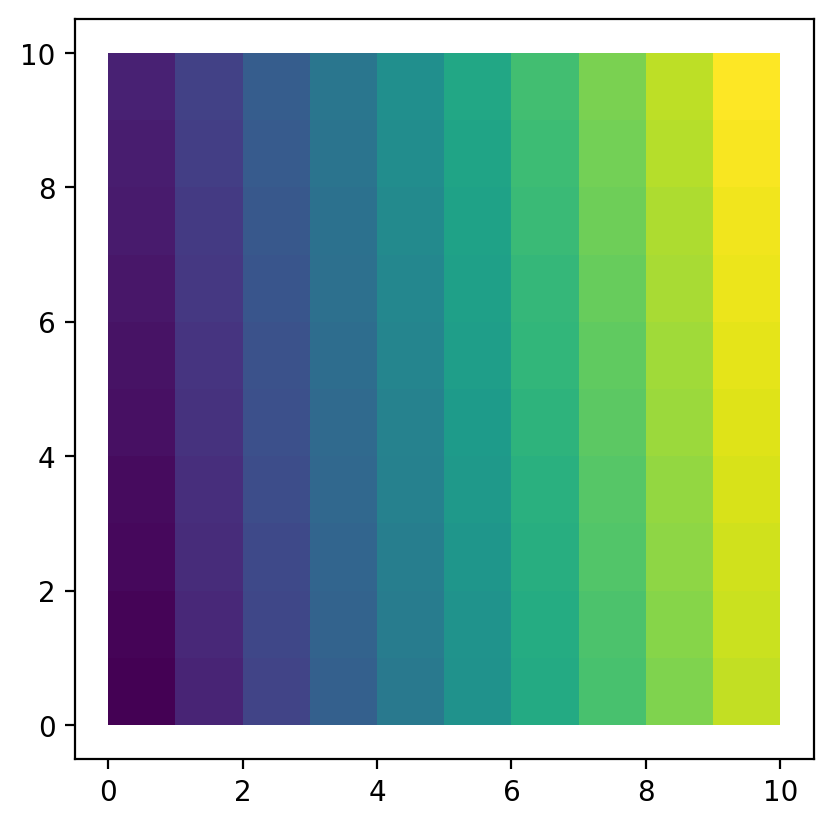
We first explore the simulated data by building a 10*10 lattice shapefile.
[8]:
libpysal.weights.build_lattice_shapefile(dim, dim, "lattice.shp")
[9]:
gdf = geopandas.read_file("lattice.shp")
gdf.plot(column="ID");
Regionalization
With reg-k-means, we aggregate 100 simulated lattices into 20 regions.
The model can then be solved:
[10]:
model = RegionKMeansHeuristic(data, 20, w)
model.solve()
[11]:
model.labels_
[11]:
array([ 2,  2,  2,  2,  2,  6, 14, 14, 19, 19, 15, 13, 13, 13, 13,  6,  6,
       14, 14, 19, 15, 15, 16, 13, 17,  6,  0,  0, 14, 19, 15, 15, 16, 18,
       18,  6,  0,  0,  0, 19, 16, 16, 16, 18,  8,  8,  0,  3, 19, 19, 10,
       10, 10, 10,  8,  3,  3,  3, 12, 12, 10,  7, 10, 10,  8,  4,  3,  3,
       12, 12,  7,  7,  7,  5,  5,  4,  4,  4, 12, 12, 11, 11, 11,  5,  5,
        1,  1,  4, 12, 12, 11, 11, 11, 11,  5,  9,  1,  1,  1,  1])
[12]:
gdf["region"] = model.labels_
gdf.plot(column="region");
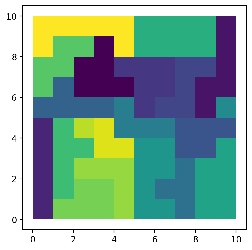
The model solution results in 20 spatially connected regions. We can summarize which lattice belongs to which region:
[13]:
areas = numpy.arange(dim * dim)
regions = [areas[model.labels_ == region] for region in range(20)]
regions
[13]:
[array([26, 27, 36, 37, 38, 46]),
 array([85, 86, 96, 97, 98, 99]),
 array([0, 1, 2, 3, 4]),
 array([47, 55, 56, 57, 66, 67]),
 array([65, 75, 76, 77, 87]),
 array([73, 74, 83, 84, 94]),
 array([ 5, 15, 16, 25, 35]),
 array([61, 70, 71, 72]),
 array([44, 45, 54, 64]),
 array([95]),
 array([50, 51, 52, 53, 60, 62, 63]),
 array([80, 81, 82, 90, 91, 92, 93]),
 array([58, 59, 68, 69, 78, 79, 88, 89]),
 array([11, 12, 13, 14, 23]),
 array([ 6,  7, 17, 18, 28]),
 array([10, 20, 21, 30, 31]),
 array([22, 32, 40, 41, 42]),
 array([24]),
 array([33, 34, 43]),
 array([ 8,  9, 19, 29, 39, 48, 49])]
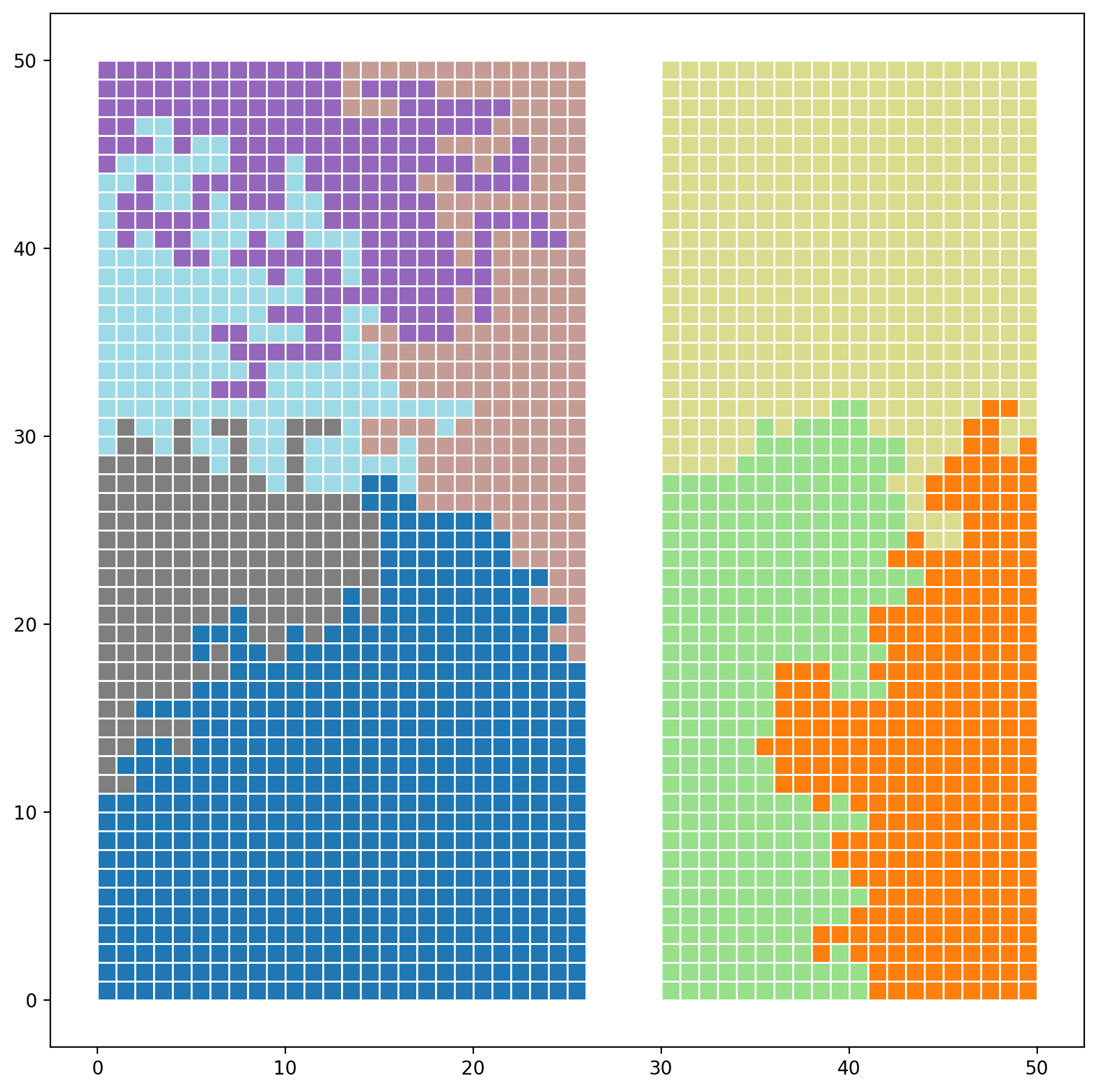
2. Large synthetic example
Create synthetic data
Generate a 50 x 50 lattice with spenc
[14]:
from spopt.region.spenclib.utils import lattice

hori, vert = 50, 50
n_polys = hori * vert
gdf = lattice(hori, vert)
gdf.head()
[14]:
| geometry | |
|---|---|
| 0 | POLYGON ((0 0, 1 0, 1 1, 0 1, 0 0)) |
| 1 | POLYGON ((0 1, 1 1, 1 2, 0 2, 0 1)) |
| 2 | POLYGON ((0 2, 1 2, 1 3, 0 3, 0 2)) |
| 3 | POLYGON ((0 3, 1 3, 1 4, 0 4, 0 3)) |
| 4 | POLYGON ((0 4, 1 4, 1 5, 0 5, 0 4)) |
Generate some random attribute data values
[15]:
numpy.random.seed(RANDOM_SEED)
gdf["data_values_1"] = numpy.random.random(n_polys)
gdf["data_values_2"] = numpy.random.random(n_polys)
vals = ["data_values_1", "data_values_2"]
gdf.head()
[15]:
| geometry | data_values_1 | data_values_2 | |
|---|---|---|---|
| 0 | POLYGON ((0 0, 1 0, 1 1, 0 1, 0 0)) | 0.929616 | 0.510240 |
| 1 | POLYGON ((0 1, 1 1, 1 2, 0 2, 0 1)) | 0.316376 | 0.483683 |
| 2 | POLYGON ((0 2, 1 2, 1 3, 0 3, 0 2)) | 0.183919 | 0.686935 |
| 3 | POLYGON ((0 3, 1 3, 1 4, 0 4, 0 3)) | 0.204560 | 0.441431 |
| 4 | POLYGON ((0 4, 1 4, 1 5, 0 5, 0 4)) | 0.567725 | 0.242545 |
Split into 2 artifical islands
[16]:
gdf = pandas.concat([gdf[:1300], gdf[1500:]], ignore_index=True)
with warnings.catch_warnings():
    warnings.filterwarnings("error")
    try:
        w = libpysal.weights.Rook.from_dataframe(gdf, use_index=False)
    except UserWarning as e:
        print(e)
        with warnings.catch_warnings():
            warnings.filterwarnings("ignore")
            w = libpysal.weights.Rook.from_dataframe(gdf, use_index=False)
The weights matrix is not fully connected:
 There are 2 disconnected components.
Regionalization
Partition into 8 regions
[17]:
numpy.random.seed(RANDOM_SEED)
model = RegionKMeansHeuristic(gdf[vals].values, 8, w)
model.solve()
[18]:
gdf["reg_k_mean"] = model.labels_
gdf.plot(
    column="reg_k_mean", categorical=True, cmap="tab20", figsize=(10, 10), edgecolor="w"
);
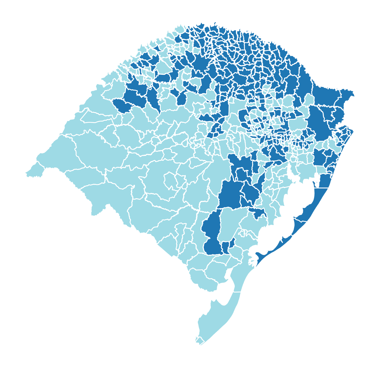
3. Empirical example (empircal geographies & synthetic atttributes)
Read in Rio Grande do Sul, Brasil dataset
[19]:
libpysal.examples.load_example("Rio Grande do Sul")
[19]:
<libpysal.examples.base.Example at 0x11f2ee630>
[20]:
rsbr = libpysal.examples.get_path("map_RS_BR.shp")
rsbr_gdf = geopandas.read_file(rsbr)
rsbr_gdf.head()
[20]:
| NM_MUNICIP | CD_GEOCMU | geometry | |
|---|---|---|---|
| 0 | ACEGUÁ | 4300034 | POLYGON ((-54.1094 -31.43316, -54.10889 -31.43... |
| 1 | ÁGUA SANTA | 4300059 | POLYGON ((-51.98932 -28.12943, -51.98901 -28.1... |
| 2 | AGUDO | 4300109 | POLYGON ((-53.13696 -29.49483, -53.13481 -29.4... |
| 3 | AJURICABA | 4300208 | POLYGON ((-53.61993 -28.14569, -53.621 -28.147... |
| 4 | ALECRIM | 4300307 | POLYGON ((-54.77813 -27.58372, -54.77307 -27.5... |
Generate some random attribute data values
[21]:
n_polys = rsbr_gdf.shape[0]
numpy.random.seed(RANDOM_SEED)
attr_cols = ["attr_1", "attr_2", "attr_3", "attr_4"]
for attr_col in attr_cols:
    rsbr_gdf[attr_col] = numpy.random.random(n_polys)
rsbr_gdf.head()
[21]:
| NM_MUNICIP | CD_GEOCMU | geometry | attr_1 | attr_2 | attr_3 | attr_4 | |
|---|---|---|---|---|---|---|---|
| 0 | ACEGUÁ | 4300034 | POLYGON ((-54.1094 -31.43316, -54.10889 -31.43... | 0.929616 | 0.990111 | 0.978448 | 0.194226 |
| 1 | ÁGUA SANTA | 4300059 | POLYGON ((-51.98932 -28.12943, -51.98901 -28.1... | 0.316376 | 0.126155 | 0.004249 | 0.245969 |
| 2 | AGUDO | 4300109 | POLYGON ((-53.13696 -29.49483, -53.13481 -29.4... | 0.183919 | 0.976601 | 0.559856 | 0.018801 |
| 3 | AJURICABA | 4300208 | POLYGON ((-53.61993 -28.14569, -53.621 -28.147... | 0.204560 | 0.229106 | 0.751780 | 0.427996 |
| 4 | ALECRIM | 4300307 | POLYGON ((-54.77813 -27.58372, -54.77307 -27.5... | 0.567725 | 0.186056 | 0.390045 | 0.179598 |
Enforce fuzzy contiguity due to nonplanar-geometries
[22]:
rsbr_w = libpysal.weights.fuzzy_contiguity(rsbr_gdf)
Partition into 2 regions
[23]:
numpy.random.seed(RANDOM_SEED)
model = RegionKMeansHeuristic(rsbr_gdf[attr_cols].values, 2, rsbr_w)
model.solve()
[24]:
rsbr_gdf["reg_k_mean"] = model.labels_
rsbr_gdf.plot(
    column="reg_k_mean", categorical=True, cmap="tab20", figsize=(8, 8), edgecolor="w"
).axis("off");