This page was generated from notebooks/p-median_variations.ipynb. Interactive online version:

Comparing P-Median Variations

This tutorial compares 4 versions of the \(p\)-median problem.

Authors

• Rongbo Xu

• Germano Barcelos

• James Gaboardi

• Levi J. Wolf

• Qunshan Zhao

Contents

1. Model data set up & inputs

2. The classic \(p\)-median problem

3. The capacited \(p\)-median problem

4. The \(k\)-nearest \(p\)-median problem

5. The capacited \(k\)-nearest \(p\)-median problem

6. Comparing variant results

7. References

Notes

• All models are solved with euclidean distance as impedence

• Detailed explanations of the classic \(p\)-median problem and the capacited variant can be found in the p-median tutorial. These models were included in spopt with GSoC 2021 by Germano Barcelos and AGILE 2023 by Rongbo Xu, respectively.

• The \(k\)-nearest \(p\)-median problem implementations were part of GSoC 2023 and contributed by Rongbo Xu. The complete, detailed write-up can be found here.

---

%config InlineBackend.figure_format = "retina"
%load_ext watermark
%watermark

Last updated: 2023-12-10T13:16:52.881916-05:00

Python implementation: CPython
Python version       : 3.12.0
IPython version      : 8.18.0

Compiler    : Clang 15.0.7
OS          : Darwin
Release     : 23.1.0
Machine     : x86_64
Processor   : i386
CPU cores   : 8
Architecture: 64bit

import geopandas
import matplotlib.colors as mcolors
import matplotlib.lines as mlines
import matplotlib.pyplot as plt
import numpy
import pandas
import pulp
import shapely
import spopt
from matplotlib.patches import Patch
from spopt.locate import KNearestPMedian, PMedian, simulated_geo_points

%watermark -w
%watermark -iv

Watermark: 2.4.3

geopandas : 0.14.1
pandas    : 2.1.3
shapely   : 2.0.2
matplotlib: 3.8.2
spopt     : 0.5.1.dev53+g5cadae7
numpy     : 1.26.2
pulp      : 2.7.0

---

1. Model data set up & inputs

Constants

• N_CLI: The quantity of client locations to simulate

• N_FAC: The quantity of facility locations to simulate

• P_FAC: Candidate facilities in an optimal solution

• SEED_CLI/SEED_FAC: Random state seeds for reproducibility

• solver: The solver engine to utilize for optimization

N_CLI = 100
N_FAC = 100
P_FAC = 5
SEED_CLI = 7
SEED_FAC = 5
solver = pulp.COIN_CMD(msg=False, warmStart=True)

---

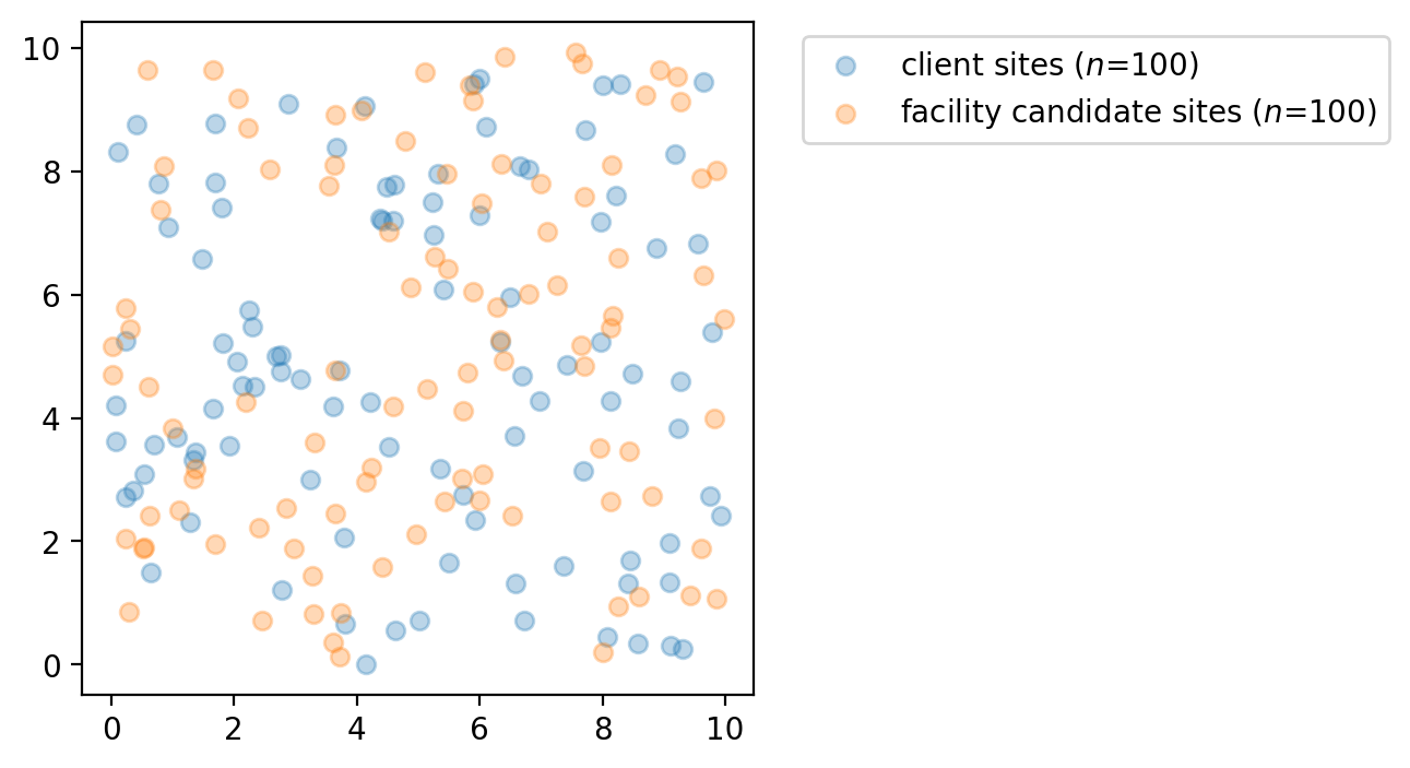
Simulate client and candidate facility locations

The simulated_geo_points utility function available in spopt simulates points in a study area.

study_area = shapely.Polygon(((0,0), (10, 0), (10,10), (0, 10)))
clients = simulated_geo_points(study_area, needed=N_CLI, seed=SEED_CLI)
facilities = simulated_geo_points(study_area, needed=N_FAC, seed=SEED_FAC)
for df in [clients, facilities]:
    df.set_crs("EPSG:4326", inplace=True)

fig, ax = plt.subplots(figsize=(4, 4))
_label = f"client sites ($n$={N_CLI})"
clients.plot(ax=ax, label=_label, alpha=.3)
_label = f"facility candidate sites ($n$={N_FAC})"
facilities.plot(ax=ax, zorder=2, label=_label, alpha=.3)
plt.legend(loc="upper left", bbox_to_anchor=(1.05, 1));

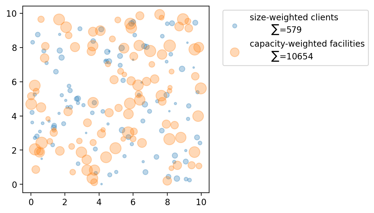
For each client location all \(p\)-median model varinates suppose there is a weight. Here we assign random integer values using numpy to simulate these weights ranging from a minimum of 1 and a maximum of 12.

numpy.random.seed(0)
ai = numpy.random.randint(1, 12, N_CLI)
clients["weights"] = ai
sum_clients = clients["weights"].sum()
print(f"The total of client weights: {sum_clients}")
clients

The total of client weights: 579

	geometry	weights
0	POINT (0.76308 7.79919)	6
1	POINT (4.38409 7.23465)	1
2	POINT (9.77990 5.38496)	4
3	POINT (5.01120 0.72051)	4
4	POINT (2.68439 4.99883)	8
...	...	...
95	POINT (1.06877 3.69486)	2
96	POINT (2.32671 4.51079)	6
97	POINT (2.76317 5.01807)	10
98	POINT (9.22603 3.82511)	4
99	POINT (6.50128 5.95621)	1

100 rows × 2 columns

For each service facility the :math:`p`-median capacitated variants suppose there is a service level available at each site (the capacity). Again, we assign random integer values using numpy to simulate these capacities ranging from a minimum of 25 and a maximum of 200.

min_cap = 25
max_cap = 200
numpy.random.seed(1)
cj = numpy.random.randint(min_cap, max_cap, N_FAC)
facilities["capacity"] = cj
sum_capacity = facilities["capacity"].sum()
print(f"The total of service capacity: {sum_capacity}")
facilities

The total of service capacity: 10654

	geometry	capacity
0	POINT (2.21993 8.70732)	62
1	POINT (2.06719 9.18611)	165
2	POINT (4.88411 6.11744)	97
3	POINT (7.65908 5.18418)	162
4	POINT (2.96801 1.87721)	158
...	...	...
95	POINT (7.26789 6.15814)	102
96	POINT (5.88500 6.05004)	100
97	POINT (3.54785 7.77382)	101
98	POINT (6.04603 3.09231)	68
99	POINT (2.45631 0.71266)	45

100 rows × 2 columns

fig, ax = plt.subplots(figsize=(4, 4))
_label = f"size-weighted clients\n\t$\\sum$={sum_clients}"
clients.plot(ax=ax, label=_label, alpha=.3, markersize=ai*4)
_label = f"capacity-weighted facilities\n\t$\\sum$={sum_capacity}"
facilities.plot(ax=ax, label=_label, alpha=.3, markersize=cj)
plt.legend(loc="upper left", bbox_to_anchor=(1.05, 1));

---

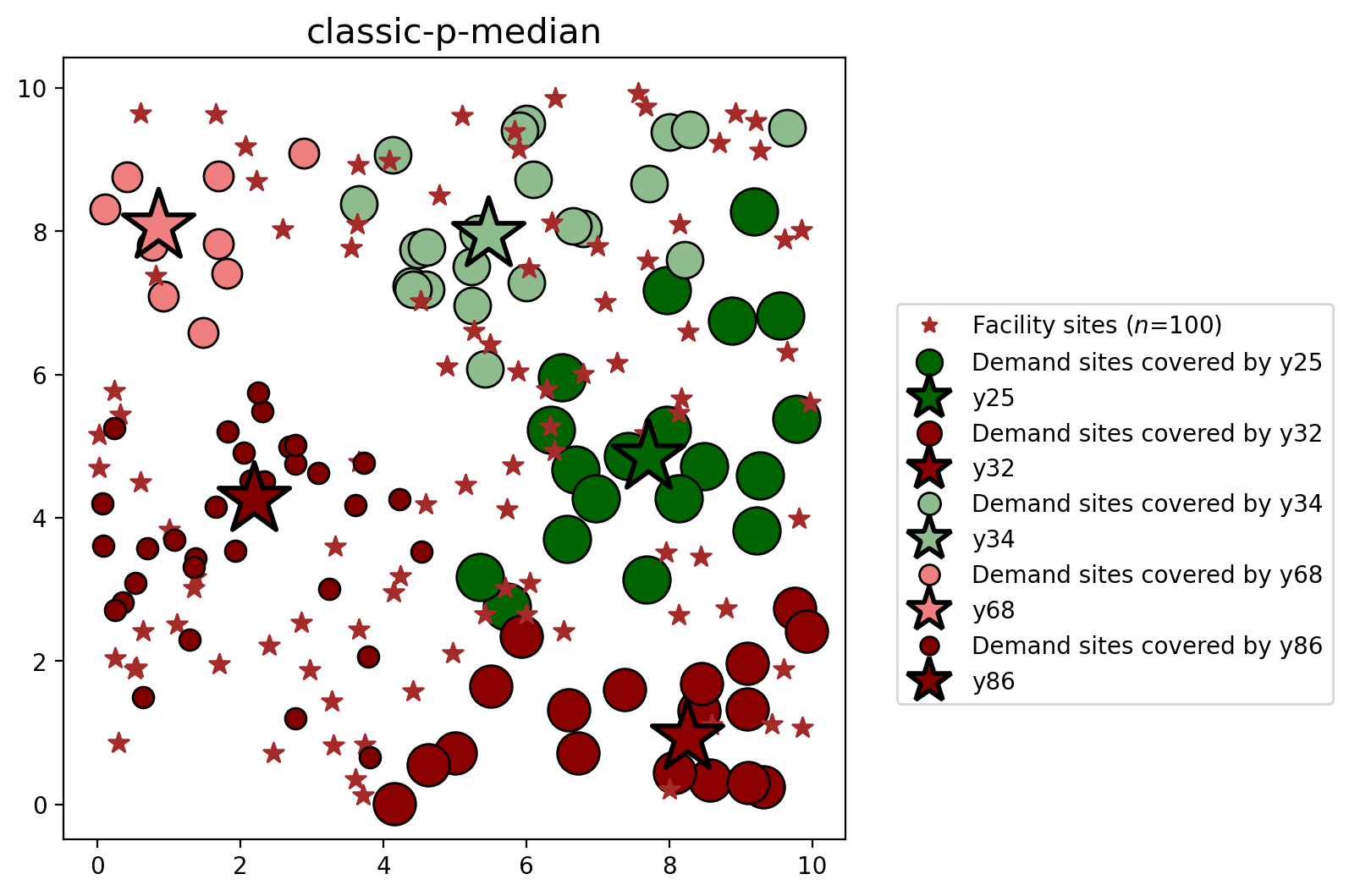
2. The classic \(p\)-median problem

The \(p\)-median problem is a classic, introduced in Hakimi (1965), seeks to minimize the maximum weights for siting \(p\) facilities. As an integer linear program (\(ILP\)), the \(p\)-median problem is formulated as:

\(\begin{array} \displaystyle \textbf{Minimize} & \displaystyle \sum_{i \in I}\sum_{j \in J}{a_i d_{ij} X_{ij}} &&& (1) \\ \displaystyle \textbf{Subject to:} & \displaystyle \sum_{j \in J}{X_{ij} = 1} & \forall i \in I && (2) \\ & \displaystyle \sum_{j \in J}{Y_{j} = p} &&& (3) \\ & X_{ij} \leq Y_{j} & \forall i \in I & \forall j \in J & (4) \\ & X_{ij} \in \{0,1\} & \forall i \in I & \forall j \in J & (5) \\ & Y_{j} \in \{0,1\} & \forall j \in J && (6) \\ \end{array}\)

\(\begin{array} \displaystyle \textbf{Where:}\\ & & \displaystyle i & \small = & \textrm{index referencing client/demand locations} \\ & & j & \small = & \textrm{index referencing potential facility sites} \\ & & d_{ij} & \small = & \textrm{shortest distance between } i \textrm{ and } j \\ & & p & \small = & \textrm{number of facilities to be located} \\ & & a_i & \small = & \textrm{service load or population demand at } i \\ & & X_{ij} & \small = & \begin{cases} 1, \textrm{if demand } i \textrm{ is assigned to facility } j \\ 0, \textrm{otherwise} \end{cases} \\ & & Y_{j} & \small = & \begin{cases} 1, \textrm{if node } j \textrm{ has been selected for a facility} \\ 0, \textrm{otherwise} \\ \end{cases} \\ \end{array}\)

The formulation above is adapted from Church and Murray (2018)

First, we declare model positional and keyword arguments, which will be used in all \(p\)-median problem variants.

model_args = clients, facilities, "geometry", "geometry", "weights", P_FAC

Instantiate and solve the classic \(p\)-median problem.

pmedian_classic = PMedian.from_geodataframe(*model_args, name="classic-p-median")
pmedian_classic = pmedian_classic.solve(solver)

Record decision variable names used for mapping later.

def fac_vars(pmp):
    return [f.name.replace("_", "") for f in pmp.fac_vars]

facilities["dv"] = fac_vars(pmedian_classic)
facilities = facilities[["geometry", "dv", "capacity"]].copy()
facilities

	geometry	dv	capacity
0	POINT (2.21993 8.70732)	y0	62
1	POINT (2.06719 9.18611)	y1	165
2	POINT (4.88411 6.11744)	y2	97
3	POINT (7.65908 5.18418)	y3	162
4	POINT (2.96801 1.87721)	y4	158
...	...	...	...
95	POINT (7.26789 6.15814)	y95	102
96	POINT (5.88500 6.05004)	y96	100
97	POINT (3.54785 7.77382)	y97	101
98	POINT (6.04603 3.09231)	y98	68
99	POINT (2.45631 0.71266)	y99	45

100 rows × 3 columns

Record solution diagnostics for model comparison.

def pmp_diagnostic(pmp, add_to=None):
    """Helper for displaying model diagnostics."""
    _diags = {
        "model": pmp.name,
        "variables": len(pmp.problem.variables()),
        "constraints": len(pmp.problem.constraints),
        "obj_val": round(pmp.problem.objective.value(), 3),
        "selected": [f.name.replace("_", "") for f in pmp.fac_vars if f.varValue],
        "cpu_time": pmp.problem.solutionCpuTime,
        "wall_time": pmp.problem.solutionTime,
    }
    _diags = pandas.DataFrame([_diags.values()], columns=_diags.keys())
    if isinstance(add_to, pandas.DataFrame):
        _diags = pandas.concat([add_to, _diags], ignore_index=True)
    return _diags

diagnostic = pmp_diagnostic(pmedian_classic)
diagnostic

	model	variables	constraints	obj_val	selected	cpu_time	wall_time
0	classic-p-median	10100	10101	906.299	[y25, y32, y34, y68, y86]	0.510654	0.921897

The classic \(p\)-median problem does not take facility capacity into account, so we can (naively) assume that 100% of the capacity at each selected candidate facility is being utilized.

def cli_sum(f2c):
    return clients.loc[f2c, "weights"].sum()

def fac_cap(fdv):
    return facilities.loc[(facilities["dv"]==fdv), "capacity"].squeeze()

def serv_perc_cap(f2c, fdv):
    return round(cli_sum(f2c) / fac_cap(fdv), 2) * 100.0

def service_level(pmp):
    if pmp.name.startswith("capacitated"):
        zipped_vars = zip(pmp.fac2cli, facilities["dv"], strict=True)
        serv_lev = [serv_perc_cap(f2c, fdv) for f2c, fdv in zipped_vars]
    else:
        serv_lev = [100.0 if bool(dv.varValue) else 0. for dv in pmp.fac_vars]
    return serv_lev

facilities["pmp_classic"] = service_level(pmedian_classic)
perc_cols = [c for c in facilities.columns if c.startswith("pmp")]
facilities.loc[(facilities[perc_cols] > 0).any(axis=1)]

	geometry	dv	capacity	pmp_classic
25	POINT (7.70854 4.84931)	y25	88	100.0
32	POINT (8.24811 0.94203)	y32	33	100.0
34	POINT (5.46358 7.96143)	y34	140	100.0
68	POINT (0.85070 8.07777)	y68	82	100.0
86	POINT (2.18498 4.25637)	y86	102	100.0

Plotting the results

dv_colors_arr = list(mcolors.CSS4_COLORS.keys())
dv_colors = {f"y{i}": dv_colors_arr[i] for i in range(len(dv_colors_arr))}

def plot_results(model, p, facs, clis=None):
    """Visualize optimal solution sets and context."""
    fig, ax = plt.subplots(figsize=(6, 6))
    markersize, markersize_factor = 4, 4
    ax.set_title(model.name, fontsize=15)

    # extract facility-client relationships for plotting
    cli_points = {}
    fac_sites = {}
    for i, dv in enumerate(model.fac_vars):
        if dv.varValue:
            dv = facs.loc[i, "dv"]
            fac_sites[dv] = i
            geom = clis.iloc[model.fac2cli[i]]["geometry"]
            cli_points[dv] = geom

    # study area and legend entries initialization
    legend_elements = []

    # all candidate facilities
    facs.plot(ax=ax, fc="brown", marker="*", markersize=80, zorder=8)
    _label = f"Facility sites ($n$={len(model.fac_vars)})"
    _mkws = dict(marker="*", markerfacecolor="brown", markeredgecolor="brown")
    legend_elements.append(mlines.Line2D([], [], ms=7, lw=0, label=_label, **_mkws))

    # facility-(client) symbology and legend entries
    zorder = 4
    for fname, fac in fac_sites.items():
        cset = dv_colors[fname]
        # clients
        geoms = cli_points[fname]
        gdf = geopandas.GeoDataFrame(geoms)
        gdf.plot(ax=ax, zorder=zorder, ec="k", fc=cset, markersize=100 * markersize)
        _label = f"Demand sites covered by {fname}"
        _mkws = dict(markerfacecolor=cset, markeredgecolor="k", ms=markersize + 7)
        legend_elements.append(
            mlines.Line2D([], [], marker="o", lw=0, label=_label, **_mkws)
        )
        # facilities
        ec = "k"
        lw = 2
        facs.iloc[[fac]].plot(
            ax=ax, marker="*", markersize=1000, zorder=9, fc=cset, ec=ec, lw=lw
        )
        _mkws = dict(markerfacecolor=cset, markeredgecolor=ec, markeredgewidth=lw)
        legend_elements.append(
            mlines.Line2D([], [], marker="*", ms=20, lw=0, label=fname, **_mkws)
        )
        # increment zorder up and markersize down for stacked client symbology
        zorder += 1
        markersize -= markersize_factor / p

    # legend
    kws = dict(loc="upper left", bbox_to_anchor=(1.05, 0.7))
    plt.legend(handles=legend_elements, **kws)

plot_results(pmedian_classic, P_FAC, facilities, clis=clients)

---

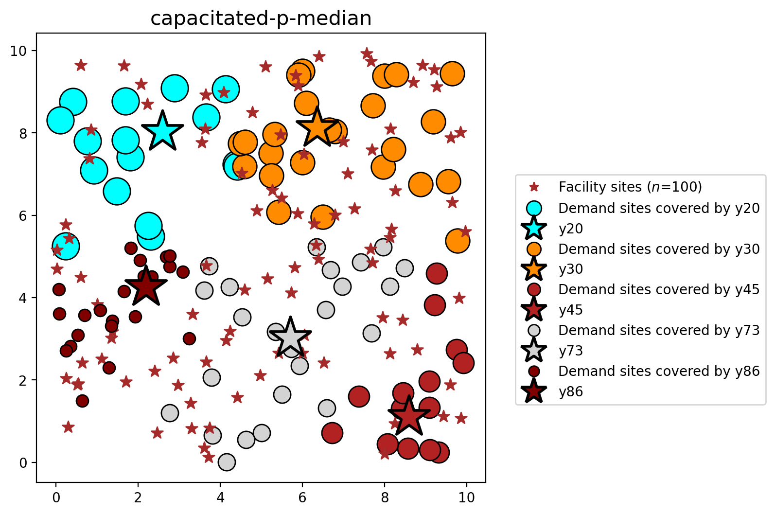
3. The capacited \(p\)-median problem

The capacitated variant of the \(p\)-median problem is formulated identically to the classic \(p\)-median problem with the addition of contraint \((4)\) below. Here constraint \((4)\) stipulates that for a facility to be considered for selection it must have the avaialable capacity to support demand from allocated client locations. The capacitated \(p\)-median variant can be formulated as:

\(\begin{array} \displaystyle \textbf{Minimize} & \displaystyle \sum_{i \in I}\sum_{j \in J}{a_i d_{ij} X_{ij}} &&& (1) \\ \displaystyle \textbf{Subject to:} & \displaystyle \sum_{j \in J}{X_{ij} = 1} & \forall i \in I && (2) \\ & \displaystyle \sum_{j \in J}{Y_{j} = p} &&& (3) \\ & \displaystyle \sum_{i \in I}{a_i X_{ij} \leq {c_j Y_{j}}}& \forall j \in J && (4) \\ & X_{ij} \leq Y_{j} & \forall i \in I & \forall j \in J & (5) \\ & X_{ij} \in \{0,1\} & \forall i \in I & \forall j \in J & (6) \\ & Y_{j} \in \{0,1\} & \forall j \in J && (7) \\ \end{array}\)

\(\begin{array} \displaystyle \textbf{Where:}\\ & & \displaystyle i & \small = & \textrm{index referencing client/demand locations} \\ & & j & \small = & \textrm{index referencing potential facility sites} \\ & & d_{ij} & \small = & \textrm{shortest distance between } i \textrm{ and } j \\ & & p & \small = & \textrm{number of facilities to be located} \\ & & a_i & \small = & \textrm{service load or population demand at } i \\ & & c_j & \small = & \textrm{capacity of facility } j \\ & & X_{ij} & \small = & \begin{cases} 1, \textrm{if demand } i \textrm{ is assigned to facility } j \\ 0, \textrm{otherwise} \end{cases} \\ & & Y_{j} & \small = & \begin{cases} 1, \textrm{if node } j \textrm{ has been selected for a facility} \\ 0, \textrm{otherwise} \\ \end{cases} \\ \end{array}\)

The formulation above is adapted from Church and Murray (2009)

pmedian_capacity = PMedian.from_geodataframe(
    *model_args, name="p-median", facility_capacity_col="capacity"
)
pmedian_capacity = pmedian_capacity.solve(solver)

diagnostic = pmp_diagnostic(pmedian_capacity, add_to=diagnostic)
diagnostic

	model	variables	constraints	obj_val	selected	cpu_time	wall_time
0	classic-p-median	10100	10101	906.299	[y25, y32, y34, y68, y86]	0.510654	0.921897
1	capacitated-p-median	10100	10201	962.151	[y20, y30, y45, y73, y86]	11.699106	12.895250

facilities["pmp_capacitated"] = service_level(pmedian_capacity)
perc_cols = [c for c in facilities.columns if c.startswith("pmp")]
facilities.loc[(facilities[perc_cols] > 0).any(axis=1)]

	geometry	dv	capacity	pmp_classic	pmp_capacitated
20	POINT (2.59098 8.02497)	y20	121	0.0	83.0
25	POINT (7.70854 4.84931)	y25	88	100.0	0.0
30	POINT (6.35356 8.11902)	y30	153	0.0	100.0
32	POINT (8.24811 0.94203)	y32	33	100.0	0.0
34	POINT (5.46358 7.96143)	y34	140	100.0	0.0
45	POINT (8.59707 1.11111)	y45	101	0.0	95.0
68	POINT (0.85070 8.07777)	y68	82	100.0	0.0
73	POINT (5.70975 3.02518)	y73	187	0.0	68.0
86	POINT (2.18498 4.25637)	y86	102	100.0	100.0

plot_results(pmedian_capacity, P_FAC, facilities, clis=clients)

---

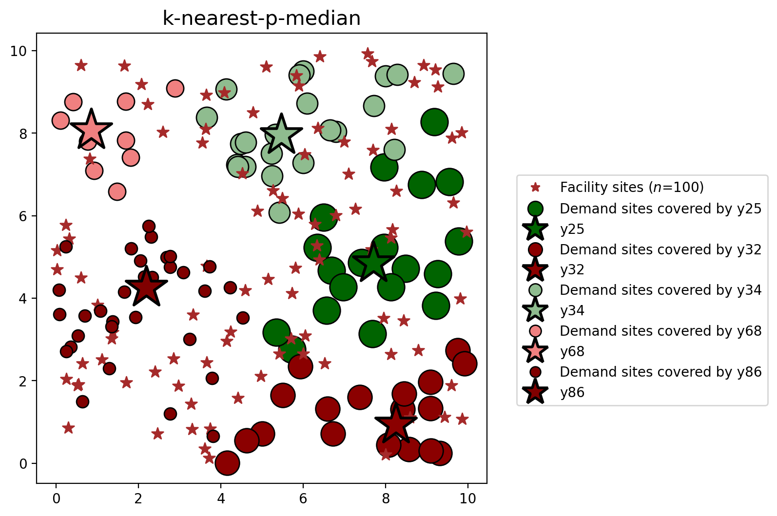
4. The \(k\)-nearest \(p\)-median problem

The \(k\)-nearest \(p\)-median problem, also referred to as the \(p\)-median model with near-far cost allocation, implements a variant of the classic \(p\)-median problem that only considers a limited selection of the nearest facilites, and was introduced in Church (2018). The focus here is the isolation a computationally efficient program for solving a \(p\)-median problem by dramatically reducing the number of variables and contraints in the mathematical formulation. As stated in the introduction above, a more detailed explanation of this model and its implementation can be found here. The \(k\)-nearest \(p\)-median variant can be formulated as:

\(\begin{array} \displaystyle \textbf{Minimize} & \displaystyle \sum_{i \in I}\sum_{k \in k_{i}}{a_i d_{ik} X_{ik}} + \sum_{i \in I}{g_i (d_{i{k_i}} + 1)} &&& (1) \\ \displaystyle \textbf{Subject to:} & \displaystyle \sum_{k \in k_{i}}{X_{ik} + g_i = 1} & \forall i \in I && (2) \\ & \displaystyle \sum_{j \in J}{Y_{j} = p} &&& (3) \\ & X_{ij} \leq Y_{j} & \forall i \in I & \forall j \in J & (4) \\ & X_{ij} \in \{0,1\} & \forall i \in I & \forall j \in J & (5) \\ & Y_{j} \in \{0,1\} & \forall j \in J && (6) \\ \end{array}\)

\(\begin{array} \displaystyle \textbf{Where:}\\ & & \displaystyle i & \small = & \textrm{index referencing client/demand locations} \\ & & j & \small = & \textrm{index referencing potential facility sites} \\ & & p & \small = & \textrm{number of facilities to be located} \\ & & a_i & \small = & \textrm{service load or population demand at } i \\ & & k_i & \small = & \textrm{the } k \textrm{ nearest facilities of client location } i \\ & & c_j & \small = & \textrm{capacity of facility } j \\ & & d_{ij} & \small = & \textrm{shortest distance between } i \textrm{ and } j \\ & & X_{ij} & \small = & \begin{cases} 1, \textrm{if demand } i \textrm{ is assigned to facility } j \\ 0, \textrm{otherwise} \end{cases} \\ & & Y_{j} & \small = & \begin{cases} 1, \textrm{if node } j \textrm{ has been selected for a facility} \\ 0, \textrm{otherwise} \\ \end{cases} \\ & & g_{i} & \small = & \begin{cases} 1, \textrm{if the client } i \textrm{ needs to be served by non-}k\textrm{-nearest facilities} \\ 0, \textrm{otherwise} \\ \end{cases} \\ \end{array}\)

The formulation above is adapted from Church (2018)

pmedian_k_nearest = KNearestPMedian.from_geodataframe(
    *model_args, name="k-nearest-p-median",
)
pmedian_k_nearest = pmedian_k_nearest.solve(solver)

diagnostic = pmp_diagnostic(pmedian_k_nearest, add_to=diagnostic)
diagnostic

	model	variables	constraints	obj_val	selected	cpu_time	wall_time
0	classic-p-median	10100	10101	906.299	[y25, y32, y34, y68, y86]	0.510654	0.921897
1	capacitated-p-median	10100	10201	962.151	[y20, y30, y45, y73, y86]	11.699106	12.895250
2	k-nearest-p-median	1598	1499	906.299	[y25, y32, y34, y68, y86]	0.064253	0.113859

facilities["pmp_k-nearest"] = service_level(pmedian_k_nearest)
perc_cols = [c for c in facilities.columns if c.startswith("pmp")]
facilities.loc[(facilities[perc_cols] > 0).any(axis=1)]

	geometry	dv	capacity	pmp_classic	pmp_capacitated	pmp_k-nearest
20	POINT (2.59098 8.02497)	y20	121	0.0	83.0	0.0
25	POINT (7.70854 4.84931)	y25	88	100.0	0.0	100.0
30	POINT (6.35356 8.11902)	y30	153	0.0	100.0	0.0
32	POINT (8.24811 0.94203)	y32	33	100.0	0.0	100.0
34	POINT (5.46358 7.96143)	y34	140	100.0	0.0	100.0
45	POINT (8.59707 1.11111)	y45	101	0.0	95.0	0.0
68	POINT (0.85070 8.07777)	y68	82	100.0	0.0	100.0
73	POINT (5.70975 3.02518)	y73	187	0.0	68.0	0.0
86	POINT (2.18498 4.25637)	y86	102	100.0	100.0	100.0

plot_results(pmedian_k_nearest, P_FAC, facilities, clis=clients)

---

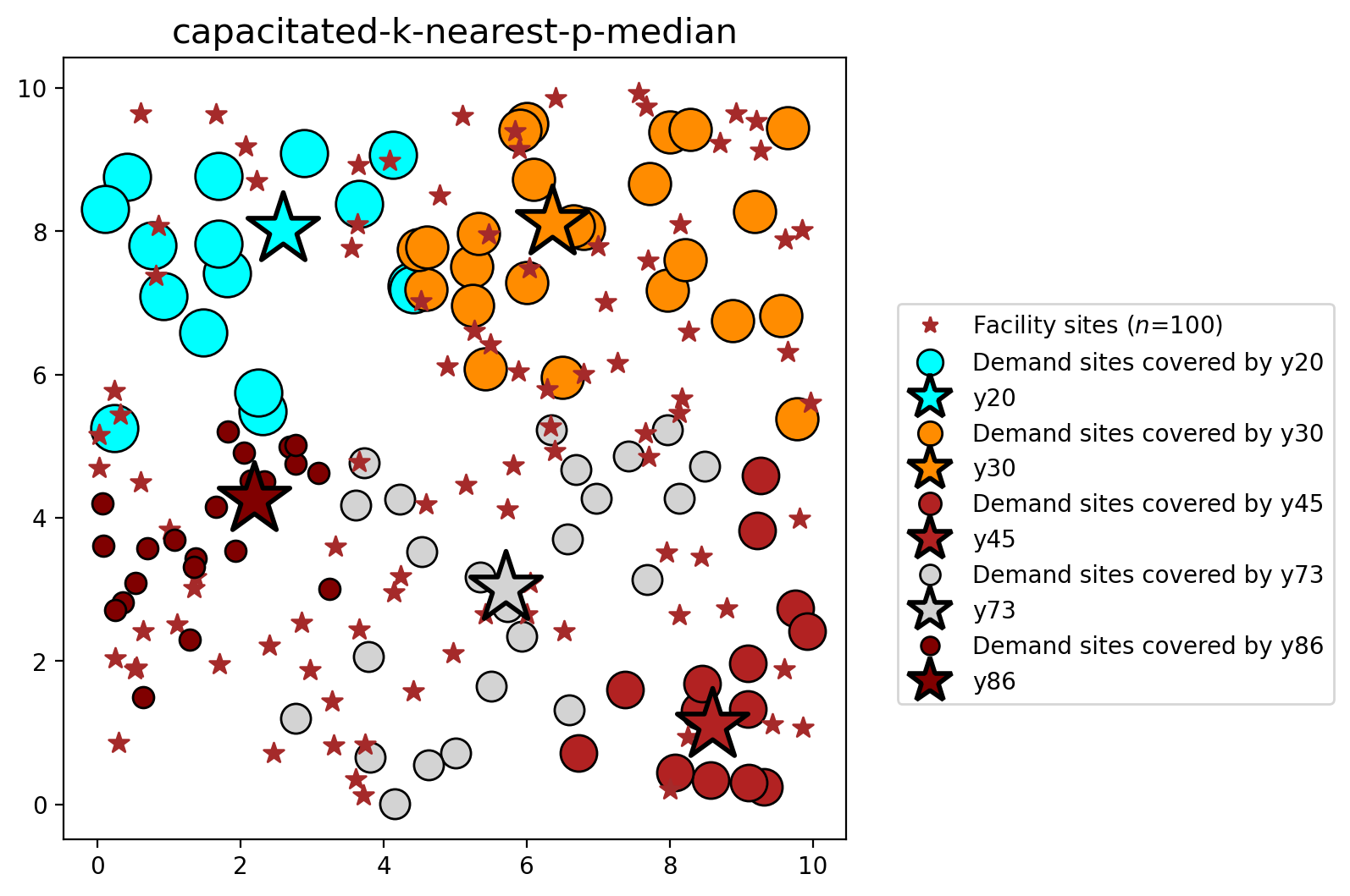
5. The capacited \(k\)-nearest \(p\)-median problem

With the addition of equation \((4)\) below, we can also introduce facility capacity as a constraint.

\(\begin{array} \displaystyle \textbf{Minimize} & \displaystyle \sum_{i \in I} \displaystyle \sum_{k \in k_{i}}{a_i d_{ik} X_{ik}} + \sum_{i \in I}{g_i (d_{i{k_i}} + 1)} &&& (1) \\ \displaystyle \textbf{Subject to:} & \displaystyle \sum_{k \in k_{i}}{X_{ik} + g_i = 1} & \forall i \in I && (2) \\ & \displaystyle \sum_{j \in J}{Y_{j} = p} &&& (3) \\ & \displaystyle \sum_{i \in I}{a_i X_{ij} \leq {c_j Y_{j}}}& \forall j \in J && (4) \\ & X_{ij} \leq Y_{j} & \forall i \in I & \forall j \in J & (5) \\ & X_{ij} \in \{0,1\} & \forall i \in I & \forall j \in J & (6) \\ & Y_{j} \in \{0,1\} & \forall j \in J && (7) \\ \end{array}\)

\(\begin{array} \displaystyle \textbf{Where:}\\ & & \displaystyle i & \small = & \textrm{index referencing client/demand locations} \\ & & j & \small = & \textrm{index referencing potential facility sites} \\ & & p & \small = & \textrm{number of facilities to be located} \\ & & a_i & \small = & \textrm{service load or population demand at } i \\ & & k_i & \small = & \textrm{the } k^{th} \textrm{nearest facilities of client location } i \\ & & c_j & \small = & \textrm{capacity of facility } j \\ & & d_{ij} & \small = & \textrm{shortest distance between } i \textrm{ and } j \\ & & X_{ij} & \small = & \begin{cases} 1, \textrm{if demand } i \textrm{ is assigned to facility } j \\ 0, \textrm{otherwise} \end{cases} \\ & & Y_{j} & \small = & \begin{cases} 1, \textrm{if node } j \textrm{ has been selected for a facility} \\ 0, \textrm{otherwise} \\ \end{cases} \\ & & g_{i} & \small = & \begin{cases} 1, \textrm{if the client } i \textrm{ needs to be served by non-k-nearest facilities} \\ 0, \textrm{otherwise} \\ \end{cases} \\ \end{array}\)

The formulation above is adapted from Church and Murray (2018)

pmedian_k_nearest_capacity = KNearestPMedian.from_geodataframe(
    *model_args,
    name="k-nearest-p-median",
    facility_capacity_col="capacity",
)
pmedian_k_nearest_capacity = pmedian_k_nearest_capacity.solve(solver)

diagnostic = pmp_diagnostic(pmedian_k_nearest_capacity, add_to=diagnostic)
diagnostic

	model	variables	constraints	obj_val	selected	cpu_time	wall_time
0	classic-p-median	10100	10101	906.299	[y25, y32, y34, y68, y86]	0.510654	0.921897
1	capacitated-p-median	10100	10201	962.151	[y20, y30, y45, y73, y86]	11.699106	12.895250
2	k-nearest-p-median	1598	1499	906.299	[y25, y32, y34, y68, y86]	0.064253	0.113859
3	capacitated-k-nearest-p-median	2045	3791	962.151	[y20, y30, y45, y73, y86]	2.610536	2.998628

facilities["pmp_k-nearest_capacitated"] = service_level(pmedian_k_nearest_capacity)
perc_cols = [c for c in facilities.columns if c.startswith("pmp")]
facilities.loc[(facilities[perc_cols] > 0).any(axis=1)]

	geometry	dv	capacity	pmp_classic	pmp_capacitated	pmp_k-nearest	pmp_k-nearest_capacitated
20	POINT (2.59098 8.02497)	y20	121	0.0	83.0	0.0	83.0
25	POINT (7.70854 4.84931)	y25	88	100.0	0.0	100.0	0.0
30	POINT (6.35356 8.11902)	y30	153	0.0	100.0	0.0	100.0
32	POINT (8.24811 0.94203)	y32	33	100.0	0.0	100.0	0.0
34	POINT (5.46358 7.96143)	y34	140	100.0	0.0	100.0	0.0
45	POINT (8.59707 1.11111)	y45	101	0.0	95.0	0.0	95.0
68	POINT (0.85070 8.07777)	y68	82	100.0	0.0	100.0	0.0
73	POINT (5.70975 3.02518)	y73	187	0.0	68.0	0.0	68.0
86	POINT (2.18498 4.25637)	y86	102	100.0	100.0	100.0	100.0

plot_results(pmedian_k_nearest_capacity, P_FAC, facilities, clis=clients)

---

6. Comparing variant results

Solution diagnostics & optimal facility selection

Below we can see that:

• The classic \(p\)-median and \(k\)-nearest variant result in equivalent objective values and facility selections. However, the \(k\)-nearest variant achieves optimality from a formulation with approximately 15% the number of variables and constraints of the classic formulation, resulting in a dramatically reduced solution time.

• Similar results are observed with the capacitated variants: equivalent objective values and facility selections, plus solve times approximately 20% faster.

• Caveat: The solve times for the \(k\)-nearest variants do not include preparation of the minimal formulation, only actual solve time reported via pulp.

diagnostic

	model	variables	constraints	obj_val	selected	cpu_time	wall_time
0	classic-p-median	10100	10101	906.299	[y25, y32, y34, y68, y86]	0.510654	0.921897
1	capacitated-p-median	10100	10201	962.151	[y20, y30, y45, y73, y86]	11.699106	12.895250
2	k-nearest-p-median	1598	1499	906.299	[y25, y32, y34, y68, y86]	0.064253	0.113859
3	capacitated-k-nearest-p-median	2045	3791	962.151	[y20, y30, y45, y73, y86]	2.610536	2.998628

facilities.loc[(facilities[perc_cols] > 0).any(axis=1)]

	geometry	dv	capacity	pmp_classic	pmp_capacitated	pmp_k-nearest	pmp_k-nearest_capacitated
20	POINT (2.59098 8.02497)	y20	121	0.0	83.0	0.0	83.0
25	POINT (7.70854 4.84931)	y25	88	100.0	0.0	100.0	0.0
30	POINT (6.35356 8.11902)	y30	153	0.0	100.0	0.0	100.0
32	POINT (8.24811 0.94203)	y32	33	100.0	0.0	100.0	0.0
34	POINT (5.46358 7.96143)	y34	140	100.0	0.0	100.0	0.0
45	POINT (8.59707 1.11111)	y45	101	0.0	95.0	0.0	95.0
68	POINT (0.85070 8.07777)	y68	82	100.0	0.0	100.0	0.0
73	POINT (5.70975 3.02518)	y73	187	0.0	68.0	0.0	68.0
86	POINT (2.18498 4.25637)	y86	102	100.0	100.0	100.0	100.0

---

7. References

• Hakimi, S. L. (1965). Optimum Distribution of Switching Centers in a Communication Network and Some Related Graph Theoretic Problems. Operations Research, 13(3), 462–475.

• Church, R. L., & Murray, A. T. (2009). Business site selection, location analysis, and GIS (pp. 209-233). Hoboken, NJ: John Wiley & Sons.

• Church, R. L. (2018). Tobler’s Law and Spatial Optimization: Why Bakersfield? International Regional Science Review, 41(3), 287–310.

• Church, R. L., & Murray, A. T. (2018). Location covering models: History, applications and advancements (1st edition 2018). Springer

---