This page was generated from notebooks/facloc-real-world.ipynb.
Interactive online version:
![]()
Empirical examples of facility location problems
Authors: Germano Barcelos, James Gaboardi, Levi J. Wolf, Qunshan Zhao
This tutorial aims to show a facility location application. To achieve this goal the tuorial will solve mulitple real world facility location problems using a dataset describing an area of census tract 205, San Francisco. The general scenarios can be stated as: store sites should supply the demand in this census tract considering the distance between the two sets of sites: demand points and candidate supply sites. Four fundamental facility location models are utilized to highlight varying outcomes dependent on objectives: LSCP (Location Set Covering Problem), MCLP (Maximal Coverage Location Problem), P-Median and P-Center. For further information on these models, it’s recommended to see the notebooks that explain more deeply about each one: LSCP, MCLP, P-Median, P-Center.
Also, this tutorial demonstrates the use of different solvers that PULP supports.
[1]:
%config InlineBackend.figure_format = "retina"
%load_ext watermark
%watermark
Last updated: 2025-04-07T13:48:14.874484-04:00

Python implementation: CPython
Python version       : 3.12.9
IPython version      : 9.0.2

Compiler    : Clang 18.1.8
OS          : Darwin
Release     : 24.4.0
Machine     : arm64
Processor   : arm
CPU cores   : 8
Architecture: 64bit
[2]:
import time
import warnings

import geopandas
import matplotlib.lines as mlines
import matplotlib.pyplot as plt
import matplotlib_scalebar
import numpy
import pandas
import pulp
import shapely
from matplotlib.patches import Patch
from matplotlib_scalebar.scalebar import ScaleBar
from shapely.geometry import Point

import spopt

%watermark -w
%watermark -iv
Watermark: 2.5.0

spopt              : 0.6.2.dev3+g13ca45e
matplotlib         : 3.10.1
pandas             : 2.2.3
numpy              : 2.2.4
matplotlib_scalebar: 0.9.0
geopandas          : 1.0.1
pulp               : 2.8.0
shapely            : 2.1.0
We use 4 data files as input:
network_distanceis the distance between facility candidate sites calculated by ArcGIS Network Analyst Extensiondemand_pointsrepresents the demand points with some important features for the facility location problem like populationfacility_pointsrepresents the stores that are candidate facility sitestractis the polygon of census tract 205.
All datasets are online on this repository.
[3]:
DIRPATH = "../spopt/tests/data/"
network_distance dataframe
[4]:
network_distance = pandas.read_csv(
    DIRPATH + "SF_network_distance_candidateStore_16_censusTract_205_new.csv"
)
network_distance
[4]:
| distance | name | DestinationName | demand | |
|---|---|---|---|---|
| 0 | 671.573346 | Store_1 | 60750479.01 | 6540 |
| 1 | 1333.708063 | Store_1 | 60750479.02 | 3539 |
| 2 | 1656.188884 | Store_1 | 60750352.02 | 4436 |
| 3 | 1783.006047 | Store_1 | 60750602.00 | 231 |
| 4 | 1790.950612 | Store_1 | 60750478.00 | 7787 |
| ... | ... | ... | ... | ... |
| 3275 | 19643.307257 | Store_19 | 60816023.00 | 3204 |
| 3276 | 20245.369594 | Store_19 | 60816029.00 | 4135 |
| 3277 | 20290.986235 | Store_19 | 60816026.00 | 7887 |
| 3278 | 20875.680521 | Store_19 | 60816025.00 | 5146 |
| 3279 | 20958.530406 | Store_19 | 60816024.00 | 6511 |
3280 rows × 4 columns
demand_points dataframe
[5]:
demand_points = pandas.read_csv(
    DIRPATH + "SF_demand_205_centroid_uniform_weight.csv", index_col=0
)
demand_points = demand_points.reset_index(drop=True)
demand_points
[5]:
| OBJECTID | ID | NAME | STATE_NAME | AREA | POP2000 | HOUSEHOLDS | HSE_UNITS | BUS_COUNT | long | lat | |
|---|---|---|---|---|---|---|---|---|---|---|---|
| 0 | 1 | 6081602900 | 60816029.00 | California | 0.48627 | 4135 | 1679 | 1715 | 112 | -122.488653 | 37.650807 |
| 1 | 2 | 6081602800 | 60816028.00 | California | 0.47478 | 4831 | 1484 | 1506 | 59 | -122.483550 | 37.659998 |
| 2 | 3 | 6081601700 | 60816017.00 | California | 0.46393 | 4155 | 1294 | 1313 | 55 | -122.456484 | 37.663272 |
| 3 | 4 | 6081601900 | 60816019.00 | California | 0.81907 | 9041 | 3273 | 3330 | 118 | -122.434247 | 37.662385 |
| 4 | 5 | 6081602500 | 60816025.00 | California | 0.46603 | 5146 | 1459 | 1467 | 44 | -122.451187 | 37.640219 |
| ... | ... | ... | ... | ... | ... | ... | ... | ... | ... | ... | ... |
| 200 | 204 | 6075011100 | 60750111.00 | California | 0.09466 | 5559 | 2930 | 3037 | 362 | -122.418479 | 37.791082 |
| 201 | 205 | 6075012200 | 60750122.00 | California | 0.07211 | 7035 | 3862 | 4074 | 272 | -122.417237 | 37.785728 |
| 202 | 206 | 6075017601 | 60750176.01 | California | 0.24306 | 5756 | 2437 | 2556 | 943 | -122.410115 | 37.779459 |
| 203 | 207 | 6075017800 | 60750178.00 | California | 0.27882 | 5829 | 3115 | 3231 | 807 | -122.405411 | 37.778934 |
| 204 | 208 | 6075012400 | 60750124.00 | California | 0.17496 | 8188 | 4328 | 4609 | 549 | -122.416455 | 37.782289 |
205 rows × 11 columns
facility_points dataframe
[6]:
facility_points = pandas.read_csv(DIRPATH + "SF_store_site_16_longlat.csv", index_col=0)
facility_points = facility_points.reset_index(drop=True)
facility_points
[6]:
| OBJECTID | NAME | long | lat | |
|---|---|---|---|---|
| 0 | 1 | Store_1 | -122.510018 | 37.772364 |
| 1 | 2 | Store_2 | -122.488873 | 37.753764 |
| 2 | 3 | Store_3 | -122.464927 | 37.774727 |
| 3 | 4 | Store_4 | -122.473945 | 37.743164 |
| 4 | 5 | Store_5 | -122.449291 | 37.731545 |
| 5 | 6 | Store_6 | -122.491745 | 37.649309 |
| 6 | 7 | Store_7 | -122.483182 | 37.701109 |
| 7 | 8 | Store_11 | -122.433782 | 37.655364 |
| 8 | 9 | Store_12 | -122.438982 | 37.719236 |
| 9 | 10 | Store_13 | -122.440218 | 37.745382 |
| 10 | 11 | Store_14 | -122.421636 | 37.742964 |
| 11 | 12 | Store_15 | -122.430982 | 37.782964 |
| 12 | 13 | Store_16 | -122.426873 | 37.769291 |
| 13 | 14 | Store_17 | -122.432345 | 37.805218 |
| 14 | 15 | Store_18 | -122.412818 | 37.805745 |
| 15 | 16 | Store_19 | -122.398909 | 37.797073 |
study_area dataframe
[7]:
study_area = geopandas.read_file(DIRPATH + "ServiceAreas_4.shp").dissolve()
study_area
[7]:
| geometry | |
|---|---|
| 0 | POLYGON ((-122.45299 37.63898, -122.45415 37.6... |
Plot study_area
[8]:
base = study_area.plot()
base.axis("off");

To start modeling the problem assuming the arguments expected by spopt.locate, we should pass a numpy 2D array as a cost matrix. So, first we pivot the network_distance dataframe.
Note that the columns and rows are sorted in ascending order.
[9]:
ntw_dist_piv = network_distance.pivot_table(
    values="distance", index="DestinationName", columns="name"
)
ntw_dist_piv
[9]:
| name | Store_1 | Store_11 | Store_12 | Store_13 | Store_14 | Store_15 | Store_16 | Store_17 | Store_18 | Store_19 | Store_2 | Store_3 | Store_4 | Store_5 | Store_6 | Store_7 |
|---|---|---|---|---|---|---|---|---|---|---|---|---|---|---|---|---|
| DestinationName | ||||||||||||||||
| 60750101.0 | 11495.190454 | 20022.666503 | 10654.593733 | 8232.543149 | 7561.399789 | 4139.772198 | 4805.805279 | 2055.530234 | 225.609240 | 1757.623456 | 11522.519829 | 7529.985950 | 10847.234951 | 10604.729605 | 20970.277793 | 15242.989416 |
| 60750102.0 | 10436.169910 | 19392.094770 | 10024.022001 | 7601.971416 | 6930.828057 | 3093.851654 | 4175.233547 | 1257.809690 | 1041.911304 | 2333.244000 | 10509.099285 | 6470.965406 | 10216.663219 | 9974.157873 | 20339.706061 | 14612.417684 |
| 60750103.0 | 10746.296811 | 19404.672860 | 10036.600090 | 7614.549505 | 6943.406146 | 3381.778555 | 4187.811636 | 2046.436590 | 744.584403 | 1685.517099 | 10800.926186 | 6778.892307 | 10229.241308 | 9986.735962 | 20352.284150 | 14624.995773 |
| 60750104.0 | 11420.492134 | 19808.368182 | 10440.295413 | 8018.244828 | 7347.101469 | 4044.473877 | 4591.506959 | 2463.736278 | 795.715285 | 1282.217412 | 11308.221508 | 7447.187630 | 10632.936630 | 10390.431285 | 20755.979472 | 15028.691095 |
| 60750105.0 | 11379.443952 | 19583.920000 | 10215.847231 | 7793.796646 | 7122.653287 | 4103.725695 | 4367.058776 | 3320.283731 | 1731.462738 | 249.669959 | 11083.773326 | 7379.539448 | 10408.488448 | 10165.983103 | 20531.531290 | 14804.242913 |
| ... | ... | ... | ... | ... | ... | ... | ... | ... | ... | ... | ... | ... | ... | ... | ... | ... |
| 60816025.0 | 17324.066610 | 2722.031291 | 10884.063331 | 14178.007937 | 13891.857275 | 18418.384867 | 16726.951785 | 20834.395022 | 21441.247824 | 20875.680521 | 14662.484617 | 16569.371114 | 12483.322114 | 11926.727459 | 4968.842581 | 8648.054204 |
| 60816026.0 | 15981.172325 | 3647.137006 | 10299.369046 | 13593.313651 | 13307.162990 | 17833.690581 | 16142.257500 | 20249.700736 | 20856.553539 | 20290.986235 | 14050.290332 | 15963.776829 | 11871.527828 | 11342.033174 | 3625.948296 | 7919.659919 |
| 60816027.0 | 14835.342712 | 4581.333336 | 9637.139433 | 12931.084039 | 12644.933377 | 17171.460969 | 15480.027887 | 19587.471124 | 20194.323926 | 19628.756623 | 13341.313338 | 15301.547216 | 11209.298215 | 10679.803561 | 2290.818683 | 7242.830306 |
| 60816028.0 | 13339.491691 | 6392.856372 | 8577.488412 | 11871.433018 | 11585.282356 | 16111.809948 | 14420.376867 | 18527.820103 | 19134.672905 | 18569.105602 | 11845.462317 | 14241.196195 | 10155.147195 | 9620.152540 | 1846.795647 | 5746.979285 |
| 60816029.0 | 15257.855684 | 6394.920365 | 10253.752405 | 13547.697010 | 13261.546349 | 17788.073940 | 16096.640859 | 20204.084095 | 20810.936898 | 20245.369594 | 13763.826309 | 15918.160188 | 11825.911187 | 11296.416533 | 508.931655 | 7665.343278 |
205 rows × 16 columns
Here the pivot table is transformed to a numpy 2D array such as spopt.locate expected. The matrix has a shape of 205x16.
[10]:
cost_matrix = ntw_dist_piv.to_numpy()
cost_matrix.shape
[10]:
(205, 16)
[11]:
cost_matrix[:3, :3]
[11]:
array([[11495.19045438, 20022.66650296, 10654.59373325],
       [10436.16991032, 19392.09477041, 10024.0220007 ],
       [10746.29681106, 19404.67285964, 10036.60008993]])
Now, as the rows and columns of our cost matrix are sorted, we have to sort our facility points and demand points geodataframes, too.
[12]:
n_dem_pnts = demand_points.shape[0]
n_fac_pnts = facility_points.shape[0]
[13]:
process = lambda df: as_gdf(df).sort_values(by=["NAME"]).reset_index(drop=True)  # noqa: E731
as_gdf = lambda df: geopandas.GeoDataFrame(df, geometry=pnts(df))  # noqa: E731
pnts = lambda df: geopandas.points_from_xy(df.long, df.lat)  # noqa: E731
[14]:
facility_points = process(facility_points)
demand_points = process(demand_points)
Reproject the input spatial data.
[15]:
for _df in [facility_points, demand_points, study_area]:
    _df.set_crs("EPSG:4326", inplace=True)
    _df.to_crs("EPSG:7131", inplace=True)
Here the rest of parameters are set.
ai is the demand weight and in this case we model as population in year 2000 of this tract.
[16]:
ai = demand_points["POP2000"].to_numpy()

# maximum service radius (in meters)
SERVICE_RADIUS = 5000

# number of candidate facilities in optimal solution
P_FACILITIES = 4
Below, the method is used to plot the results of the four models that we will prepare to solve the problem.
[17]:
dv_colors_arr = [
    "darkcyan",
    "mediumseagreen",
    "saddlebrown",
    "darkslategray",
    "lightskyblue",
    "thistle",
    "lavender",
    "darkgoldenrod",
    "peachpuff",
    "coral",
    "mediumvioletred",
    "blueviolet",
    "fuchsia",
    "cyan",
    "limegreen",
    "mediumorchid",
]
dv_colors = {f"y{i}": dv_colors_arr[i] for i in range(len(dv_colors_arr))}
dv_colors
[17]:
{'y0': 'darkcyan',
 'y1': 'mediumseagreen',
 'y2': 'saddlebrown',
 'y3': 'darkslategray',
 'y4': 'lightskyblue',
 'y5': 'thistle',
 'y6': 'lavender',
 'y7': 'darkgoldenrod',
 'y8': 'peachpuff',
 'y9': 'coral',
 'y10': 'mediumvioletred',
 'y11': 'blueviolet',
 'y12': 'fuchsia',
 'y13': 'cyan',
 'y14': 'limegreen',
 'y15': 'mediumorchid'}
[18]:
def plot_results(model, p, facs, clis=None, ax=None):
    """Visualize optimal solution sets and context."""
    if not ax:
        multi_plot = False
        fig, ax = plt.subplots(figsize=(6, 9))
        markersize, markersize_factor = 4, 4
    else:
        ax.axis("off")
        multi_plot = True
        markersize, markersize_factor = 2, 2
    ax.set_title(model.name, fontsize=15)

    # extract facility-client relationships for plotting (except for p-dispersion)
    plot_clis = isinstance(clis, geopandas.GeoDataFrame)
    if plot_clis:
        cli_points = {}
    fac_sites = {}
    for i, dv in enumerate(model.fac_vars):
        if dv.varValue:
            dv, predef = facs.loc[i, ["dv", "predefined_loc"]]
            fac_sites[dv] = [i, predef]
            if plot_clis:
                geom = clis.iloc[model.fac2cli[i]]["geometry"]
                cli_points[dv] = geom

    # study area and legend entries initialization
    study_area.plot(ax=ax, alpha=0.5, fc="tan", ec="k", zorder=1)
    _patch = Patch(alpha=0.5, fc="tan", ec="k", label="Dissolved Service Areas")
    legend_elements = [_patch]

    if plot_clis and model.name.startswith("mclp"):
        # any clients that not asscociated with a facility
        c = "k"
        if model.n_cli_uncov:
            idx = [i for i, v in enumerate(model.cli2fac) if len(v) == 0]
            pnt_kws = {
                "ax": ax,
                "fc": c,
                "ec": c,
                "marker": "s",
                "markersize": 7,
                "zorder": 2,
            }
            clis.iloc[idx].plot(**pnt_kws)
        _label = f"Demand sites not covered ($n$={model.n_cli_uncov})"
        _mkws = {
            "marker": "s",
            "markerfacecolor": c,
            "markeredgecolor": c,
            "linewidth": 0,
        }
        legend_elements.append(mlines.Line2D([], [], ms=3, label=_label, **_mkws))

    # all candidate facilities
    facs.plot(ax=ax, fc="brown", marker="*", markersize=80, zorder=8)
    _label = f"Facility sites ($n$={len(model.fac_vars)})"
    _mkws = {"marker": "*", "markerfacecolor": "brown", "markeredgecolor": "brown"}
    legend_elements.append(mlines.Line2D([], [], ms=7, lw=0, label=_label, **_mkws))

    # facility-(client) symbology and legend entries
    zorder = 4
    for fname, (fac, predef) in fac_sites.items():
        cset = dv_colors[fname]
        if plot_clis:
            # clients
            geoms = cli_points[fname]
            gdf = geopandas.GeoDataFrame(geoms)
            gdf.plot(ax=ax, zorder=zorder, ec="k", fc=cset, markersize=100 * markersize)
            _label = f"Demand sites covered by {fname}"
            _mkws = {
                "markerfacecolor": cset,
                "markeredgecolor": "k",
                "ms": markersize + 7,
            }
            legend_elements.append(
                mlines.Line2D([], [], marker="o", lw=0, label=_label, **_mkws)
            )
        # facilities
        ec = "k"
        lw = 2
        predef_label = "predefined"
        if model.name.endswith(predef_label) and predef:
            ec = "r"
            lw = 3
            fname += f" ({predef_label})"
        facs.iloc[[fac]].plot(
            ax=ax, marker="*", markersize=1000, zorder=9, fc=cset, ec=ec, lw=lw
        )
        _mkws = {"markerfacecolor": cset, "markeredgecolor": ec, "markeredgewidth": lw}
        legend_elements.append(
            mlines.Line2D([], [], marker="*", ms=20, lw=0, label=fname, **_mkws)
        )
        # increment zorder up and markersize down for stacked client symbology
        zorder += 1
        if plot_clis:
            markersize -= markersize_factor / p

    if not multi_plot:
        # legend
        kws = {"loc": "upper left", "bbox_to_anchor": (1.05, 0.7)}
        plt.legend(handles=legend_elements, **kws)
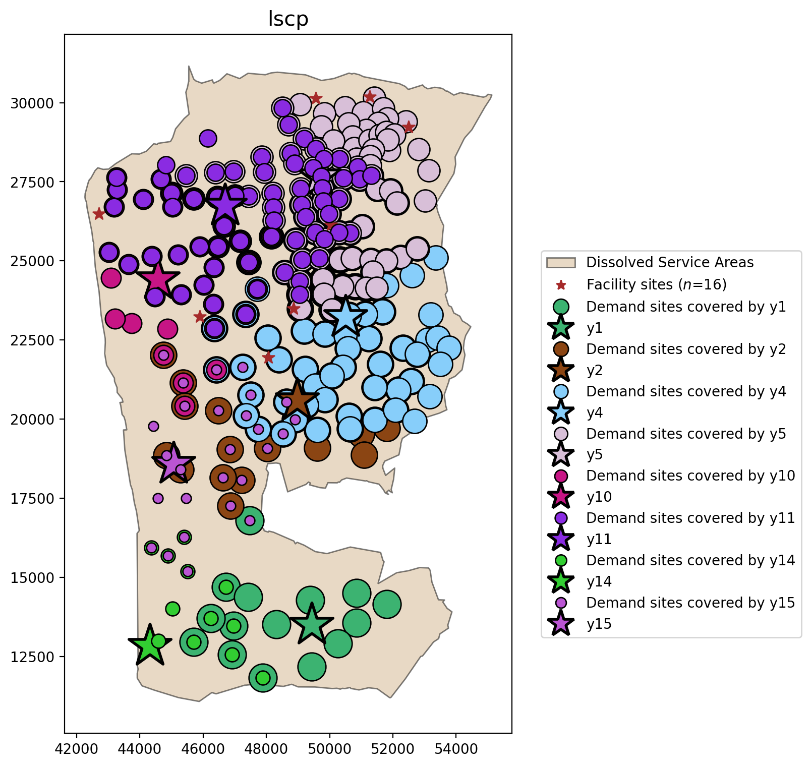
LSCP
[19]:
from spopt.locate import LSCP

lscp = LSCP.from_cost_matrix(cost_matrix, SERVICE_RADIUS)
lscp = lscp.solve(pulp.GLPK(msg=False))
lscp_objval = lscp.problem.objective.value()
lscp_objval
[19]:
8
Define the decision variable names used for mapping.
[20]:
facility_points["dv"] = lscp.fac_vars
facility_points["dv"] = facility_points["dv"].map(lambda x: x.name.replace("_", ""))
facility_points["predefined_loc"] = 0
[21]:
plot_results(lscp, lscp_objval, facility_points, clis=demand_points)
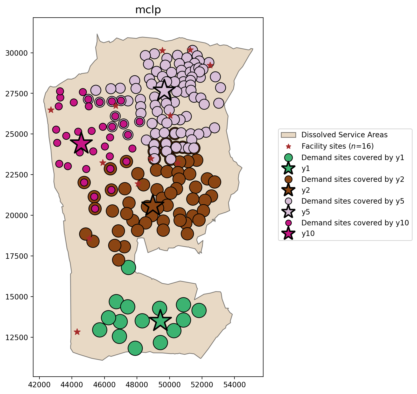
MCLP
[22]:
from spopt.locate import MCLP

mclp = MCLP.from_cost_matrix(
    cost_matrix,
    ai,
    service_radius=SERVICE_RADIUS,
    p_facilities=P_FACILITIES,
)
mclp = mclp.solve(pulp.GLPK(msg=False))
mclp.problem.objective.value()
[22]:
875247
MCLP Percentage Covered
[23]:
mclp.perc_cov
[23]:
89.75609756097562
[24]:
plot_results(mclp, P_FACILITIES, facility_points, clis=demand_points)
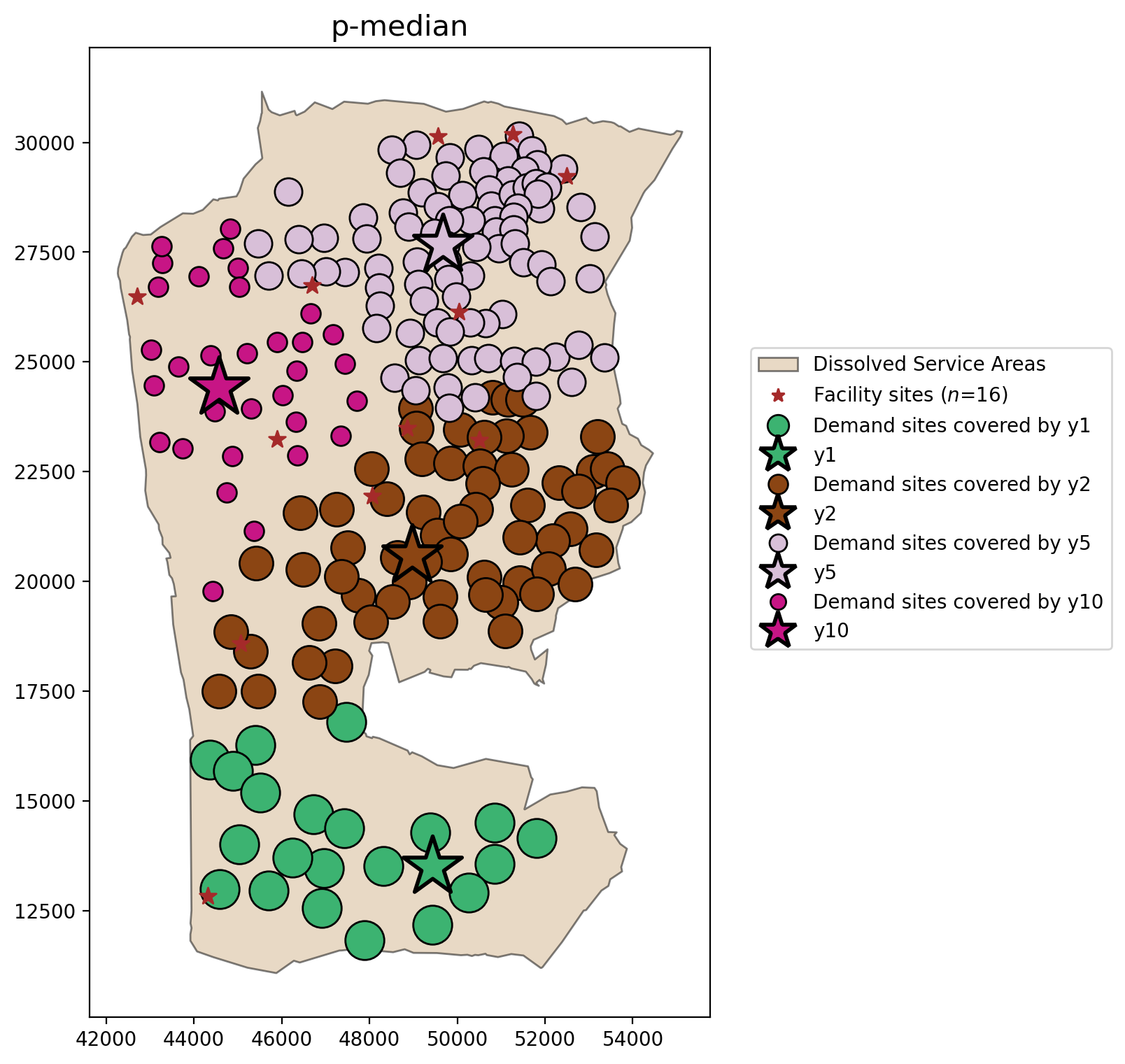
P-Median
[25]:
from spopt.locate import PMedian

pmedian = PMedian.from_cost_matrix(cost_matrix, ai, p_facilities=P_FACILITIES)
pmedian = pmedian.solve(pulp.GLPK(msg=False))
pmedian.problem.objective.value()
[25]:
2848268129.7145104
\(p\)-median mean weighted distance
[26]:
pmedian.mean_dist
[26]:
np.float64(2982.1268579890657)
[27]:
plot_results(pmedian, P_FACILITIES, facility_points, clis=demand_points)
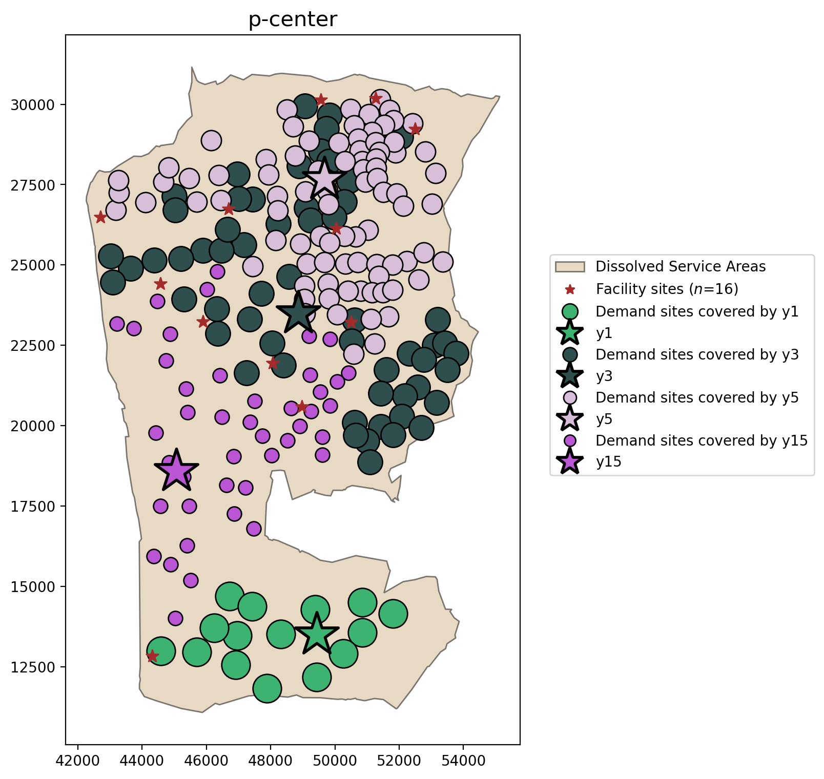
P-Center
[28]:
from spopt.locate import PCenter

pcenter = PCenter.from_cost_matrix(cost_matrix, p_facilities=P_FACILITIES)
pcenter = pcenter.solve(pulp.GLPK(msg=False))
pcenter.problem.objective.value()
[28]:
7403.06
[29]:
plot_results(pcenter, P_FACILITIES, facility_points, clis=demand_points)
Comparing all models
[30]:
fig, axarr = plt.subplots(1, 4, figsize=(20, 10))
fig.subplots_adjust(wspace=-0.01)
for i, m in enumerate([lscp, mclp, pmedian, pcenter]):
    _p = m.problem.objective.value() if m.name == "lscp" else P_FACILITIES
    plot_results(m, _p, facility_points, clis=demand_points, ax=axarr[i])

The plot above clearly demonstrates the key features of each location model:
LSCP
Overlapping clusters of clients associated with multiple facilities
All clients covered by at least one facility
MCLP
Overlapping clusters of clients associated with multiple facilities
Potential for complete coverage, but not guranteed
\(p\)-median
Tight and distinct clusters of client-facility relationships
All clients allocated to exactly one facility
\(p\)-center
Loose and overlapping clusters of client-facility relationships
All clients allocated to exactly one facility
Evaluating available solvers
For this task we’ll solve the MCLP and \(p\)-center models as examples of solver performance, but first we’ll determine which solvers are installed locally.
[31]:
with warnings.catch_warnings(record=True) as w:
    solvers = pulp.listSolvers(onlyAvailable=True)
for _w in w:
    print(_w.message)
solvers
[31]:
['GLPK_CMD', 'PULP_CBC_CMD', 'COIN_CMD', 'SCIP_CMD', 'HiGHS', 'HiGHS_CMD']
Above we can see that it returns a list with different solvers that are available. So, it’s up to the user to choose the best solver that fits the model.
MCLP
Let’s get the percentage as a metric to evaluate which solver is the best or improves the model.
[32]:
mclp = MCLP.from_cost_matrix(
    cost_matrix,
    ai,
    service_radius=SERVICE_RADIUS,
    p_facilities=P_FACILITIES,
)
[33]:
results = pandas.DataFrame(columns=["Coverage %", "Solve Time (sec.)"], index=solvers)
for solver in solvers:
    _mclp = mclp.solve(pulp.getSolver(solver, msg=False))
    results.loc[solver] = [_mclp.perc_cov, _mclp.problem.solutionTime]
results
Running HiGHS 1.10.0 (git hash: n/a): Copyright (c) 2025 HiGHS under MIT licence terms
MIP  has 206 rows; 221 cols; 1128 nonzeros; 221 integer variables (221 binary)
Coefficient ranges:
  Matrix [1e+00, 1e+00]
  Cost   [1e+02, 9e+03]
  Bound  [1e+00, 1e+00]
  RHS    [4e+00, 4e+00]
Presolving model
206 rows, 221 cols, 1128 nonzeros  0s
206 rows, 221 cols, 1128 nonzeros  0s
Objective function is integral with scale 1

Solving MIP model with:
   206 rows
   221 cols (221 binary, 0 integer, 0 implied int., 0 continuous)
   1128 nonzeros

Src: B => Branching; C => Central rounding; F => Feasibility pump; H => Heuristic; L => Sub-MIP;
     P => Empty MIP; R => Randomized rounding; S => Solve LP; T => Evaluate node; U => Unbounded;
     z => Trivial zero; l => Trivial lower; u => Trivial upper; p => Trivial point; X => User solution

        Nodes      |    B&B Tree     |            Objective Bounds              |  Dynamic Constraints |       Work
Src  Proc. InQueue |  Leaves   Expl. | BestBound       BestSol              Gap |   Cuts   InLp Confl. | LpIters     Time

         0       0         0   0.00%   -955113         inf                  inf        0      0      0         0     0.0s
 T       0       0         0   0.00%   -955113         -875247            9.12%        0      0      0        58     0.0s
         1       0         1 100.00%   -875247         -875247            0.00%        0      0      0        58     0.0s

Solving report
  Status            Optimal
  Primal bound      -875247
  Dual bound        -875247
  Gap               0% (tolerance: 0.01%)
  P-D integral      1.22046566357e-06
  Solution status   feasible
                    -875247 (objective)
                    0 (bound viol.)
                    0 (int. viol.)
                    0 (row viol.)
  Timing            0.00 (total)
                    0.00 (presolve)
                    0.00 (solve)
                    0.00 (postsolve)
  Max sub-MIP depth 0
  Nodes             1
  Repair LPs        0 (0 feasible; 0 iterations)
  LP iterations     58 (total)
                    0 (strong br.)
                    0 (separation)
                    0 (heuristics)
[33]:
| Coverage % | Solve Time (sec.) | |
|---|---|---|
| GLPK_CMD | 89.756098 | 0.012869 |
| PULP_CBC_CMD | 89.756098 | 0.051969 |
| COIN_CMD | 89.756098 | 0.039173 |
| SCIP_CMD | 89.756098 | 0.060814 |
| HiGHS | 89.756098 | 0.004004 |
| HiGHS_CMD | 89.756098 | 0.022751 |
As is expected from such a small model the Coverage %, and thus the objective values, are equivalent for all solutions across solvers. However, solve times do vary slightly.
P-Center
[34]:
pcenter = PCenter.from_cost_matrix(cost_matrix, p_facilities=P_FACILITIES)
[35]:
results = pandas.DataFrame(columns=["MinMax", "Solve Time (sec.)"], index=solvers)
for solver in solvers:
    _pcenter = pcenter.solve(pulp.getSolver(solver, msg=False))
    results.loc[solver] = [
        _pcenter.problem.objective.value(),
        _pcenter.problem.solutionTime,
    ]
results
Running HiGHS 1.10.0 (git hash: n/a): Copyright (c) 2025 HiGHS under MIT licence terms
MIP  has 3691 rows; 3297 cols; 13341 nonzeros; 3296 integer variables (3296 binary)
Coefficient ranges:
  Matrix [1e+00, 2e+04]
  Cost   [1e+00, 1e+00]
  Bound  [1e+00, 1e+00]
  RHS    [1e+00, 4e+00]
Presolving model
3691 rows, 3297 cols, 13341 nonzeros  0s
3691 rows, 3297 cols, 13294 nonzeros  0s

Solving MIP model with:
   3691 rows
   3297 cols (3296 binary, 0 integer, 0 implied int., 1 continuous)
   13294 nonzeros

Src: B => Branching; C => Central rounding; F => Feasibility pump; H => Heuristic; L => Sub-MIP;
     P => Empty MIP; R => Randomized rounding; S => Solve LP; T => Evaluate node; U => Unbounded;
     z => Trivial zero; l => Trivial lower; u => Trivial upper; p => Trivial point; X => User solution

        Nodes      |    B&B Tree     |            Objective Bounds              |  Dynamic Constraints |       Work
Src  Proc. InQueue |  Leaves   Expl. | BestBound       BestSol              Gap |   Cuts   InLp Confl. | LpIters     Time

         0       0         0   0.00%   996.5383584     inf                  inf        0      0      0         0     0.0s
 R       0       0         0   0.00%   4785.978168     20022.666503      76.10%        0      0      0      1777     0.1s
 L       0       0         0   0.00%   5039.133055     7853.410078       35.84%     1731    183      0      2584     0.7s

0.2% inactive integer columns, restarting
Model after restart has 3685 rows, 3291 cols (3290 bin., 0 int., 0 impl., 1 cont.), and 13270 nonzeros

         0       0         0   0.00%   5039.133055     7853.410078       35.84%       42      0      0      4806     0.7s
         0       0         0   0.00%   5039.133055     7853.410078       35.84%       42     29      1      6395     0.8s
 L       0       0         0   0.00%   5438.977261     7685.736909       29.23%     1009     61      2      8409     1.0s

12.5% inactive integer columns, restarting
Model after restart has 2065 rows, 1713 cols (1712 bin., 0 int., 0 impl., 1 cont.), and 6922 nonzeros

         0       0         0   0.00%   5438.977261     7685.736909       29.23%       18      0      0      9277     1.0s
 R       0       0         0   0.00%   5490.658256     7640.121657       28.13%       18      6      0     11177     1.0s
 L       0       0         0   0.00%   7287.145024     7403.063811        1.57%     3893     46      0     21202     1.7s
         1       0         1 100.00%   7403.063811     7403.063811        0.00%     3719     46      0     21325     1.7s

Solving report
  Status            Optimal
  Primal bound      7403.06381085
  Dual bound        7403.06381085
  Gap               0% (tolerance: 0.01%)
  P-D integral      0.646976539781
  Solution status   feasible
                    7403.06381085 (objective)
                    0 (bound viol.)
                    0 (int. viol.)
                    0 (row viol.)
  Timing            1.71 (total)
                    0.00 (presolve)
                    0.00 (solve)
                    0.00 (postsolve)
  Max sub-MIP depth 1
  Nodes             1
  Repair LPs        0 (0 feasible; 0 iterations)
  LP iterations     21325 (total)
                    0 (strong br.)
                    12855 (separation)
                    3081 (heuristics)
[35]:
| MinMax | Solve Time (sec.) | |
|---|---|---|
| GLPK_CMD | 7403.06 | 14.192957 |
| PULP_CBC_CMD | 7403.0638 | 1.104676 |
| COIN_CMD | 7403.0638 | 1.026668 |
| SCIP_CMD | 7403.063811 | 1.807097 |
| HiGHS | 7403.063811 | 1.734226 |
| HiGHS_CMD | 7403.063811 | 1.505336 |
Here the MinMax objective values are mostly equivalent, but there are some precision concerns. This is due to the computational complexity of the \(p\)-center problem, which also results in dramaticaly longer run times needed to isolate the optimal solutions (when compared with the MCLP above).