This page was generated from notebooks/facloc-lscpb-real-world.ipynb.
Interactive online version:
![]()
Backup Coverage Location Problem: An Empirical Example
Authors: Erin Olson, Germano Barcelos, James Gaboardi, Levi J. Wolf, Qunshan Zhao
This tutorial extends the Empirical examples notebook, specifically for the Backup Coverage Location Set Covering Problem (LSCP-B). A deeper dive into the LSCP-B can be found here. Also, this tutorial demonstrates the use of different solvers that PULP supports.
[1]:
%config InlineBackend.figure_format = "retina"
%load_ext watermark
%watermark
Last updated: 2025-04-07T13:52:13.732102-04:00

Python implementation: CPython
Python version       : 3.12.9
IPython version      : 9.0.2

Compiler    : Clang 18.1.8
OS          : Darwin
Release     : 24.4.0
Machine     : arm64
Processor   : arm
CPU cores   : 8
Architecture: 64bit
[2]:
import time
import warnings

import geopandas
import matplotlib.lines as mlines
import matplotlib.pyplot as plt
import matplotlib_scalebar
import pandas
import pulp
import shapely
from matplotlib.patches import Patch
from matplotlib_scalebar.scalebar import ScaleBar
from shapely.geometry import Point

import spopt
from spopt.locate import LSCP, LSCPB

%watermark -w
%watermark -iv
Watermark: 2.5.0

shapely            : 2.1.0
matplotlib_scalebar: 0.9.0
pulp               : 2.8.0
matplotlib         : 3.10.1
spopt              : 0.6.2.dev3+g13ca45e
geopandas          : 1.0.1
pandas             : 2.2.3
We use 4 data files as input:
network_distanceis the distance between facility candidate sites calculated by ArcGIS Network Analyst Extensiondemand_pointsrepresents the demand points with some important features for the facility location problem like populationfacility_pointsrepresents the stores that are candidate facility sitestractis the polygon of census tract 205.
All datasets are online on this repository.
[3]:
DIRPATH = "../spopt/tests/data/"
network_distance dataframe
[4]:
network_distance = pandas.read_csv(
    DIRPATH + "SF_network_distance_candidateStore_16_censusTract_205_new.csv"
)
network_distance
[4]:
| distance | name | DestinationName | demand | |
|---|---|---|---|---|
| 0 | 671.573346 | Store_1 | 60750479.01 | 6540 |
| 1 | 1333.708063 | Store_1 | 60750479.02 | 3539 |
| 2 | 1656.188884 | Store_1 | 60750352.02 | 4436 |
| 3 | 1783.006047 | Store_1 | 60750602.00 | 231 |
| 4 | 1790.950612 | Store_1 | 60750478.00 | 7787 |
| ... | ... | ... | ... | ... |
| 3275 | 19643.307257 | Store_19 | 60816023.00 | 3204 |
| 3276 | 20245.369594 | Store_19 | 60816029.00 | 4135 |
| 3277 | 20290.986235 | Store_19 | 60816026.00 | 7887 |
| 3278 | 20875.680521 | Store_19 | 60816025.00 | 5146 |
| 3279 | 20958.530406 | Store_19 | 60816024.00 | 6511 |
3280 rows × 4 columns
demand_points dataframe
[5]:
demand_points = pandas.read_csv(
    DIRPATH + "SF_demand_205_centroid_uniform_weight.csv", index_col=0
)
demand_points = demand_points.reset_index(drop=True)
demand_points
[5]:
| OBJECTID | ID | NAME | STATE_NAME | AREA | POP2000 | HOUSEHOLDS | HSE_UNITS | BUS_COUNT | long | lat | |
|---|---|---|---|---|---|---|---|---|---|---|---|
| 0 | 1 | 6081602900 | 60816029.00 | California | 0.48627 | 4135 | 1679 | 1715 | 112 | -122.488653 | 37.650807 |
| 1 | 2 | 6081602800 | 60816028.00 | California | 0.47478 | 4831 | 1484 | 1506 | 59 | -122.483550 | 37.659998 |
| 2 | 3 | 6081601700 | 60816017.00 | California | 0.46393 | 4155 | 1294 | 1313 | 55 | -122.456484 | 37.663272 |
| 3 | 4 | 6081601900 | 60816019.00 | California | 0.81907 | 9041 | 3273 | 3330 | 118 | -122.434247 | 37.662385 |
| 4 | 5 | 6081602500 | 60816025.00 | California | 0.46603 | 5146 | 1459 | 1467 | 44 | -122.451187 | 37.640219 |
| ... | ... | ... | ... | ... | ... | ... | ... | ... | ... | ... | ... |
| 200 | 204 | 6075011100 | 60750111.00 | California | 0.09466 | 5559 | 2930 | 3037 | 362 | -122.418479 | 37.791082 |
| 201 | 205 | 6075012200 | 60750122.00 | California | 0.07211 | 7035 | 3862 | 4074 | 272 | -122.417237 | 37.785728 |
| 202 | 206 | 6075017601 | 60750176.01 | California | 0.24306 | 5756 | 2437 | 2556 | 943 | -122.410115 | 37.779459 |
| 203 | 207 | 6075017800 | 60750178.00 | California | 0.27882 | 5829 | 3115 | 3231 | 807 | -122.405411 | 37.778934 |
| 204 | 208 | 6075012400 | 60750124.00 | California | 0.17496 | 8188 | 4328 | 4609 | 549 | -122.416455 | 37.782289 |
205 rows × 11 columns
facility_points dataframe
[6]:
facility_points = pandas.read_csv(DIRPATH + "SF_store_site_16_longlat.csv", index_col=0)
facility_points = facility_points.reset_index(drop=True)
facility_points
[6]:
| OBJECTID | NAME | long | lat | |
|---|---|---|---|---|
| 0 | 1 | Store_1 | -122.510018 | 37.772364 |
| 1 | 2 | Store_2 | -122.488873 | 37.753764 |
| 2 | 3 | Store_3 | -122.464927 | 37.774727 |
| 3 | 4 | Store_4 | -122.473945 | 37.743164 |
| 4 | 5 | Store_5 | -122.449291 | 37.731545 |
| 5 | 6 | Store_6 | -122.491745 | 37.649309 |
| 6 | 7 | Store_7 | -122.483182 | 37.701109 |
| 7 | 8 | Store_11 | -122.433782 | 37.655364 |
| 8 | 9 | Store_12 | -122.438982 | 37.719236 |
| 9 | 10 | Store_13 | -122.440218 | 37.745382 |
| 10 | 11 | Store_14 | -122.421636 | 37.742964 |
| 11 | 12 | Store_15 | -122.430982 | 37.782964 |
| 12 | 13 | Store_16 | -122.426873 | 37.769291 |
| 13 | 14 | Store_17 | -122.432345 | 37.805218 |
| 14 | 15 | Store_18 | -122.412818 | 37.805745 |
| 15 | 16 | Store_19 | -122.398909 | 37.797073 |
study_area dataframe
[7]:
study_area = geopandas.read_file(DIRPATH + "ServiceAreas_4.shp").dissolve()
study_area
[7]:
| geometry | |
|---|---|
| 0 | POLYGON ((-122.45299 37.63898, -122.45415 37.6... |
Plot study_area
[8]:
base = study_area.plot()
base.axis("off");

To start modeling the problem assuming the arguments expected by spopt.locate, we should pass a numpy 2D array as a cost matrix. So, first we pivot the network_distance dataframe.
Note that the columns and rows are sorted in ascending order.
[9]:
ntw_dist_piv = network_distance.pivot_table(
    values="distance", index="DestinationName", columns="name"
)
ntw_dist_piv
[9]:
| name | Store_1 | Store_11 | Store_12 | Store_13 | Store_14 | Store_15 | Store_16 | Store_17 | Store_18 | Store_19 | Store_2 | Store_3 | Store_4 | Store_5 | Store_6 | Store_7 |
|---|---|---|---|---|---|---|---|---|---|---|---|---|---|---|---|---|
| DestinationName | ||||||||||||||||
| 60750101.0 | 11495.190454 | 20022.666503 | 10654.593733 | 8232.543149 | 7561.399789 | 4139.772198 | 4805.805279 | 2055.530234 | 225.609240 | 1757.623456 | 11522.519829 | 7529.985950 | 10847.234951 | 10604.729605 | 20970.277793 | 15242.989416 |
| 60750102.0 | 10436.169910 | 19392.094770 | 10024.022001 | 7601.971416 | 6930.828057 | 3093.851654 | 4175.233547 | 1257.809690 | 1041.911304 | 2333.244000 | 10509.099285 | 6470.965406 | 10216.663219 | 9974.157873 | 20339.706061 | 14612.417684 |
| 60750103.0 | 10746.296811 | 19404.672860 | 10036.600090 | 7614.549505 | 6943.406146 | 3381.778555 | 4187.811636 | 2046.436590 | 744.584403 | 1685.517099 | 10800.926186 | 6778.892307 | 10229.241308 | 9986.735962 | 20352.284150 | 14624.995773 |
| 60750104.0 | 11420.492134 | 19808.368182 | 10440.295413 | 8018.244828 | 7347.101469 | 4044.473877 | 4591.506959 | 2463.736278 | 795.715285 | 1282.217412 | 11308.221508 | 7447.187630 | 10632.936630 | 10390.431285 | 20755.979472 | 15028.691095 |
| 60750105.0 | 11379.443952 | 19583.920000 | 10215.847231 | 7793.796646 | 7122.653287 | 4103.725695 | 4367.058776 | 3320.283731 | 1731.462738 | 249.669959 | 11083.773326 | 7379.539448 | 10408.488448 | 10165.983103 | 20531.531290 | 14804.242913 |
| ... | ... | ... | ... | ... | ... | ... | ... | ... | ... | ... | ... | ... | ... | ... | ... | ... |
| 60816025.0 | 17324.066610 | 2722.031291 | 10884.063331 | 14178.007937 | 13891.857275 | 18418.384867 | 16726.951785 | 20834.395022 | 21441.247824 | 20875.680521 | 14662.484617 | 16569.371114 | 12483.322114 | 11926.727459 | 4968.842581 | 8648.054204 |
| 60816026.0 | 15981.172325 | 3647.137006 | 10299.369046 | 13593.313651 | 13307.162990 | 17833.690581 | 16142.257500 | 20249.700736 | 20856.553539 | 20290.986235 | 14050.290332 | 15963.776829 | 11871.527828 | 11342.033174 | 3625.948296 | 7919.659919 |
| 60816027.0 | 14835.342712 | 4581.333336 | 9637.139433 | 12931.084039 | 12644.933377 | 17171.460969 | 15480.027887 | 19587.471124 | 20194.323926 | 19628.756623 | 13341.313338 | 15301.547216 | 11209.298215 | 10679.803561 | 2290.818683 | 7242.830306 |
| 60816028.0 | 13339.491691 | 6392.856372 | 8577.488412 | 11871.433018 | 11585.282356 | 16111.809948 | 14420.376867 | 18527.820103 | 19134.672905 | 18569.105602 | 11845.462317 | 14241.196195 | 10155.147195 | 9620.152540 | 1846.795647 | 5746.979285 |
| 60816029.0 | 15257.855684 | 6394.920365 | 10253.752405 | 13547.697010 | 13261.546349 | 17788.073940 | 16096.640859 | 20204.084095 | 20810.936898 | 20245.369594 | 13763.826309 | 15918.160188 | 11825.911187 | 11296.416533 | 508.931655 | 7665.343278 |
205 rows × 16 columns
Here the pivot table is transformed to numpy 2D array such as spopt.locate expected. The matrix has a shape of 205x16.
[10]:
cost_matrix = ntw_dist_piv.to_numpy()
cost_matrix.shape
[10]:
(205, 16)
[11]:
cost_matrix[:3, :3]
[11]:
array([[11495.19045438, 20022.66650296, 10654.59373325],
       [10436.16991032, 19392.09477041, 10024.0220007 ],
       [10746.29681106, 19404.67285964, 10036.60008993]])
Now, as the rows and columns of our cost matrix are sorted, we have to sort our facility points and demand points geodataframes, too.
[12]:
n_dem_pnts = demand_points.shape[0]
n_fac_pnts = facility_points.shape[0]
[13]:
process = lambda df: as_gdf(df).sort_values(by=["NAME"]).reset_index(drop=True)  # noqa: E731
as_gdf = lambda df: geopandas.GeoDataFrame(df, geometry=pnts(df))  # noqa: E731
pnts = lambda df: geopandas.points_from_xy(df.long, df.lat)  # noqa: E731
[14]:
facility_points = process(facility_points)
demand_points = process(demand_points)
Reproject the input spatial data.
[15]:
for _df in [facility_points, demand_points, study_area]:
    _df.set_crs("EPSG:4326", inplace=True)
    _df.to_crs("EPSG:7131", inplace=True)
Set parameter SERVICE_RADIUS for maximum service standard of distance or time.
[16]:
# maximum service radius (in meters)
SERVICE_RADIUS = 8000
[17]:
solver = pulp.PULP_CBC_CMD(msg=False)
LSCP & LSCP-B considering all candidate facilities
[18]:
lscp = LSCP.from_cost_matrix(cost_matrix, SERVICE_RADIUS)
lscp = lscp.solve(solver)
[19]:
lscpb = LSCPB.from_cost_matrix(cost_matrix, SERVICE_RADIUS, solver)
lscpb = lscpb.solve()
[20]:
lscp_obj = lscp.problem.objective.value()
lscpb_obj = lscpb.problem.objective.value()
lscpb_lscp = lscpb.lscp_obj_value
lscpb_perc = round(lscpb.backup_perc, 3)
print(
    "The minimum number of facilites needed to achieve complete "
    f"coverage within a distance units service radius of {SERVICE_RADIUS} "
    f"are {lscp_obj} and {lscpb_lscp} for the LSCP and LSCP-B, "
    "respectively. However, with the LSCP-B we observe coverage by more "
    f"than one facility at {lscpb_perc}% of client locations."
)
The minimum number of facilites needed to achieve complete coverage within a distance units service radius of 8000 are 3.0 and 3.0 for the LSCP and LSCP-B, respectively. However, with the LSCP-B we observe coverage by more than one facility at 69.756% of client locations.
Define the decision variable names used for mapping later.
[21]:
facility_points["dv"] = lscpb.fac_vars
facility_points["dv"] = facility_points["dv"].map(
    lambda x: x.name.replace("_", "").replace("x", "y")
)
facility_points
[21]:
| OBJECTID | NAME | long | lat | geometry | dv | |
|---|---|---|---|---|---|---|
| 0 | 1 | Store_1 | -122.510018 | 37.772364 | POINT (42712.165 26483.898) | y0 |
| 1 | 8 | Store_11 | -122.433782 | 37.655364 | POINT (49431.133 13496.279) | y1 |
| 2 | 9 | Store_12 | -122.438982 | 37.719236 | POINT (48971.439 20585.532) | y2 |
| 3 | 10 | Store_13 | -122.440218 | 37.745382 | POINT (48862.129 23487.462) | y3 |
| 4 | 11 | Store_14 | -122.421636 | 37.742964 | POINT (50499.936 23219.396) | y4 |
| 5 | 12 | Store_15 | -122.430982 | 37.782964 | POINT (49675.336 27658.898) | y5 |
| 6 | 13 | Store_16 | -122.426873 | 37.769291 | POINT (50037.687 26141.402) | y6 |
| 7 | 14 | Store_17 | -122.432345 | 37.805218 | POINT (49554.745 30128.981) | y7 |
| 8 | 15 | Store_18 | -122.412818 | 37.805745 | POINT (51274.389 30188.01) | y8 |
| 9 | 16 | Store_19 | -122.398909 | 37.797073 | POINT (52499.809 29225.972) | y9 |
| 10 | 2 | Store_2 | -122.488873 | 37.753764 | POINT (44574.304 24418.447) | y10 |
| 11 | 3 | Store_3 | -122.464927 | 37.774727 | POINT (46684.891 26744.653) | y11 |
| 12 | 4 | Store_4 | -122.473945 | 37.743164 | POINT (45889.483 23241.485) | y12 |
| 13 | 5 | Store_5 | -122.449291 | 37.731545 | POINT (48062.508 21951.687) | y13 |
| 14 | 6 | Store_6 | -122.491745 | 37.649309 | POINT (44315.976 12824.977) | y14 |
| 15 | 7 | Store_7 | -122.483182 | 37.701109 | POINT (45073.75 18574.015) | y15 |
LSCP & LSCP-B with selection of predefined candidate facilities
However, in many real world applications there may already be existing facility locations with the goal being to add one or more new facilities. Here we will define facilites \(y_{11}\) and \(y_{15}\) as already existing (they must be present in the model solution). This will lead to a sub-optimal solution.
Important: The facilities in "predefined_loc" are a binary array where 1 means the associated location must appear in the solution.
[22]:
facility_points["predefined_loc"] = 0
facility_points.loc[(11, 15), "predefined_loc"] = 1
facility_points
[22]:
| OBJECTID | NAME | long | lat | geometry | dv | predefined_loc | |
|---|---|---|---|---|---|---|---|
| 0 | 1 | Store_1 | -122.510018 | 37.772364 | POINT (42712.165 26483.898) | y0 | 0 |
| 1 | 8 | Store_11 | -122.433782 | 37.655364 | POINT (49431.133 13496.279) | y1 | 0 |
| 2 | 9 | Store_12 | -122.438982 | 37.719236 | POINT (48971.439 20585.532) | y2 | 0 |
| 3 | 10 | Store_13 | -122.440218 | 37.745382 | POINT (48862.129 23487.462) | y3 | 0 |
| 4 | 11 | Store_14 | -122.421636 | 37.742964 | POINT (50499.936 23219.396) | y4 | 0 |
| 5 | 12 | Store_15 | -122.430982 | 37.782964 | POINT (49675.336 27658.898) | y5 | 0 |
| 6 | 13 | Store_16 | -122.426873 | 37.769291 | POINT (50037.687 26141.402) | y6 | 0 |
| 7 | 14 | Store_17 | -122.432345 | 37.805218 | POINT (49554.745 30128.981) | y7 | 0 |
| 8 | 15 | Store_18 | -122.412818 | 37.805745 | POINT (51274.389 30188.01) | y8 | 0 |
| 9 | 16 | Store_19 | -122.398909 | 37.797073 | POINT (52499.809 29225.972) | y9 | 0 |
| 10 | 2 | Store_2 | -122.488873 | 37.753764 | POINT (44574.304 24418.447) | y10 | 0 |
| 11 | 3 | Store_3 | -122.464927 | 37.774727 | POINT (46684.891 26744.653) | y11 | 1 |
| 12 | 4 | Store_4 | -122.473945 | 37.743164 | POINT (45889.483 23241.485) | y12 | 0 |
| 13 | 5 | Store_5 | -122.449291 | 37.731545 | POINT (48062.508 21951.687) | y13 | 0 |
| 14 | 6 | Store_6 | -122.491745 | 37.649309 | POINT (44315.976 12824.977) | y14 | 0 |
| 15 | 7 | Store_7 | -122.483182 | 37.701109 | POINT (45073.75 18574.015) | y15 | 1 |
[23]:
lscp_pre = LSCP.from_cost_matrix(
    cost_matrix,
    SERVICE_RADIUS,
    predefined_facilities_arr=facility_points["predefined_loc"].values,
    name="lscp-predefined",
)
lscp_pre = lscp_pre.solve(solver)
[24]:
lscpb_pre = LSCPB.from_cost_matrix(
    cost_matrix,
    SERVICE_RADIUS,
    solver=solver,
    predefined_facilities_arr=facility_points["predefined_loc"].values,
    name="lscp-b-predefined",
)
lscpb_pre = lscpb_pre.solve()
[25]:
lscp_obj = lscp_pre.problem.objective.value()
lscpb_obj = lscpb_pre.problem.objective.value()
lscpb_lscp = lscpb_pre.lscp_obj_value
lscpb_perc = round(lscpb_pre.backup_perc, 3)
print(
    "The minimum number of facilites needed to achieve complete "
    f"coverage within a distance units service radius of {SERVICE_RADIUS} "
    f"are {lscp_obj} and {lscpb_lscp} for the LSCP and LSCP-B, "
    "respectively. However, with the LSCP-B we observe coverage by more "
    f"than one facility at {lscpb_perc}% of client locations."
)
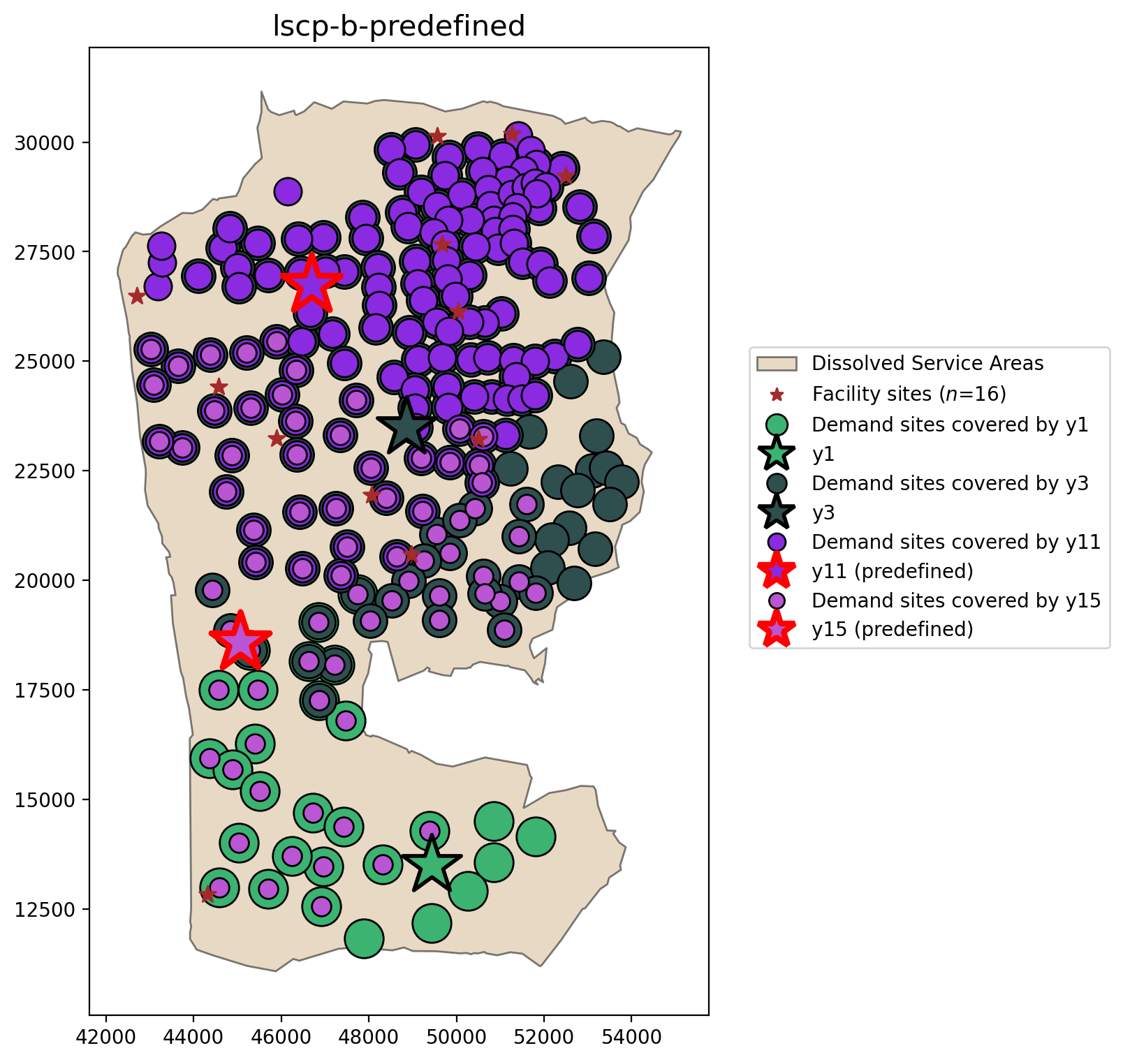
The minimum number of facilites needed to achieve complete coverage within a distance units service radius of 8000 are 4.0 and 4.0 for the LSCP and LSCP-B, respectively. However, with the LSCP-B we observe coverage by more than one facility at 87.805% of client locations.
Plotting the results
[26]:
dv_colors_arr = [
    "darkcyan",
    "mediumseagreen",
    "saddlebrown",
    "darkslategray",
    "lightskyblue",
    "thistle",
    "lavender",
    "darkgoldenrod",
    "peachpuff",
    "coral",
    "mediumvioletred",
    "blueviolet",
    "fuchsia",
    "cyan",
    "limegreen",
    "mediumorchid",
]
dv_colors = {f"y{i}": dv_colors_arr[i] for i in range(len(dv_colors_arr))}
dv_colors
[26]:
{'y0': 'darkcyan',
 'y1': 'mediumseagreen',
 'y2': 'saddlebrown',
 'y3': 'darkslategray',
 'y4': 'lightskyblue',
 'y5': 'thistle',
 'y6': 'lavender',
 'y7': 'darkgoldenrod',
 'y8': 'peachpuff',
 'y9': 'coral',
 'y10': 'mediumvioletred',
 'y11': 'blueviolet',
 'y12': 'fuchsia',
 'y13': 'cyan',
 'y14': 'limegreen',
 'y15': 'mediumorchid'}
[27]:
def plot_results(model, p, facs, clis=None, ax=None):
    """Visualize optimal solution sets and context."""
    if not ax:
        multi_plot = False
        fig, ax = plt.subplots(figsize=(6, 9))
        markersize, markersize_factor = 4, 4
    else:
        ax.axis("off")
        multi_plot = True
        markersize, markersize_factor = 2, 2
    ax.set_title(model.name, fontsize=15)

    # extract facility-client relationships for plotting (except for p-dispersion)
    plot_clis = isinstance(clis, geopandas.GeoDataFrame)
    if plot_clis:
        cli_points = {}
    fac_sites = {}
    for i, dv in enumerate(model.fac_vars):
        if dv.varValue:
            dv, predef = facs.loc[i, ["dv", "predefined_loc"]]
            fac_sites[dv] = [i, predef]
            if plot_clis:
                geom = clis.iloc[model.fac2cli[i]]["geometry"]
                cli_points[dv] = geom

    # study area and legend entries initialization
    study_area.plot(ax=ax, alpha=0.5, fc="tan", ec="k", zorder=1)
    _patch = Patch(alpha=0.5, fc="tan", ec="k", label="Dissolved Service Areas")
    legend_elements = [_patch]

    if plot_clis and model.name.startswith("mclp"):
        # any clients that not asscociated with a facility
        c = "k"
        if model.n_cli_uncov:
            idx = [i for i, v in enumerate(model.cli2fac) if len(v) == 0]
            pnt_kws = {
                "ax": ax,
                "fc": c,
                "ec": c,
                "marker": "s",
                "markersize": 7,
                "zorder": 2,
            }
            clis.iloc[idx].plot(**pnt_kws)
        _label = f"Demand sites not covered ($n$={model.n_cli_uncov})"
        _mkws = {
            "marker": "s",
            "markerfacecolor": c,
            "markeredgecolor": c,
            "linewidth": 0,
        }
        legend_elements.append(mlines.Line2D([], [], ms=3, label=_label, **_mkws))

    # all candidate facilities
    facs.plot(ax=ax, fc="brown", marker="*", markersize=80, zorder=8)
    _label = f"Facility sites ($n$={len(model.fac_vars)})"
    _mkws = {"marker": "*", "markerfacecolor": "brown", "markeredgecolor": "brown"}
    legend_elements.append(mlines.Line2D([], [], ms=7, lw=0, label=_label, **_mkws))

    # facility-(client) symbology and legend entries
    zorder = 4
    for fname, (fac, predef) in fac_sites.items():
        cset = dv_colors[fname]
        if plot_clis:
            # clients
            geoms = cli_points[fname]
            gdf = geopandas.GeoDataFrame(geoms)
            gdf.plot(ax=ax, zorder=zorder, ec="k", fc=cset, markersize=100 * markersize)
            _label = f"Demand sites covered by {fname}"
            _mkws = {
                "markerfacecolor": cset,
                "markeredgecolor": "k",
                "ms": markersize + 7,
            }
            legend_elements.append(
                mlines.Line2D([], [], marker="o", lw=0, label=_label, **_mkws)
            )
        # facilities
        ec = "k"
        lw = 2
        predef_label = "predefined"
        if model.name.endswith(predef_label) and predef:
            ec = "r"
            lw = 3
            fname += f" ({predef_label})"
        facs.iloc[[fac]].plot(
            ax=ax, marker="*", markersize=1000, zorder=9, fc=cset, ec=ec, lw=lw
        )
        _mkws = {"markerfacecolor": cset, "markeredgecolor": ec, "markeredgewidth": lw}
        legend_elements.append(
            mlines.Line2D([], [], marker="*", ms=20, lw=0, label=fname, **_mkws)
        )
        # increment zorder up and markersize down for stacked client symbology
        zorder += 1
        if plot_clis:
            markersize -= markersize_factor / p

    if not multi_plot:
        # legend
        kws = {"loc": "upper left", "bbox_to_anchor": (1.05, 0.7)}
        plt.legend(handles=legend_elements, **kws)
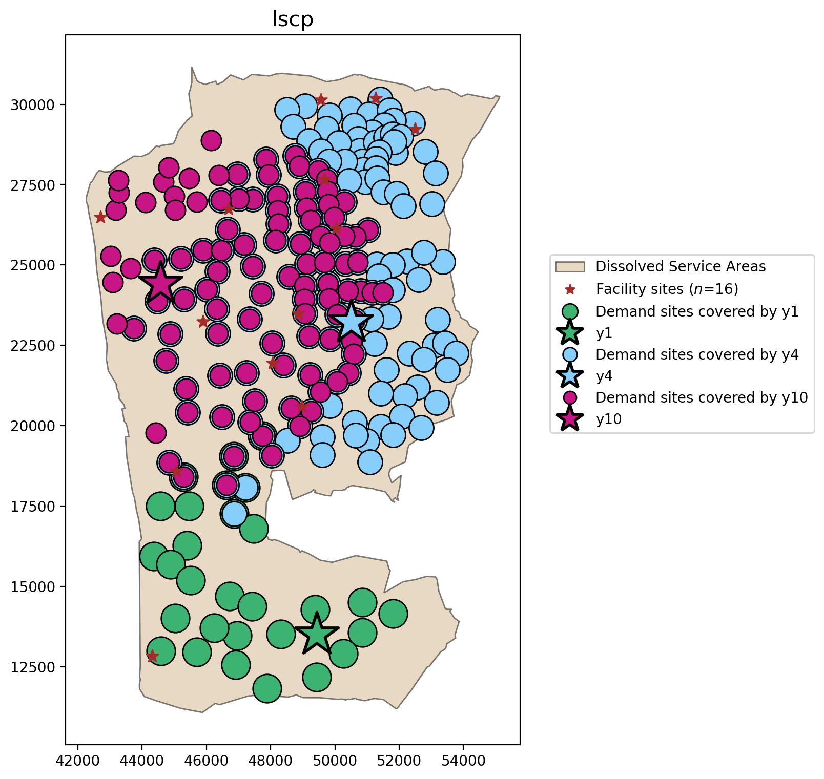
LSCP considering all candidate facilities
[28]:
plot_results(lscp, lscp_obj, facility_points, clis=demand_points)
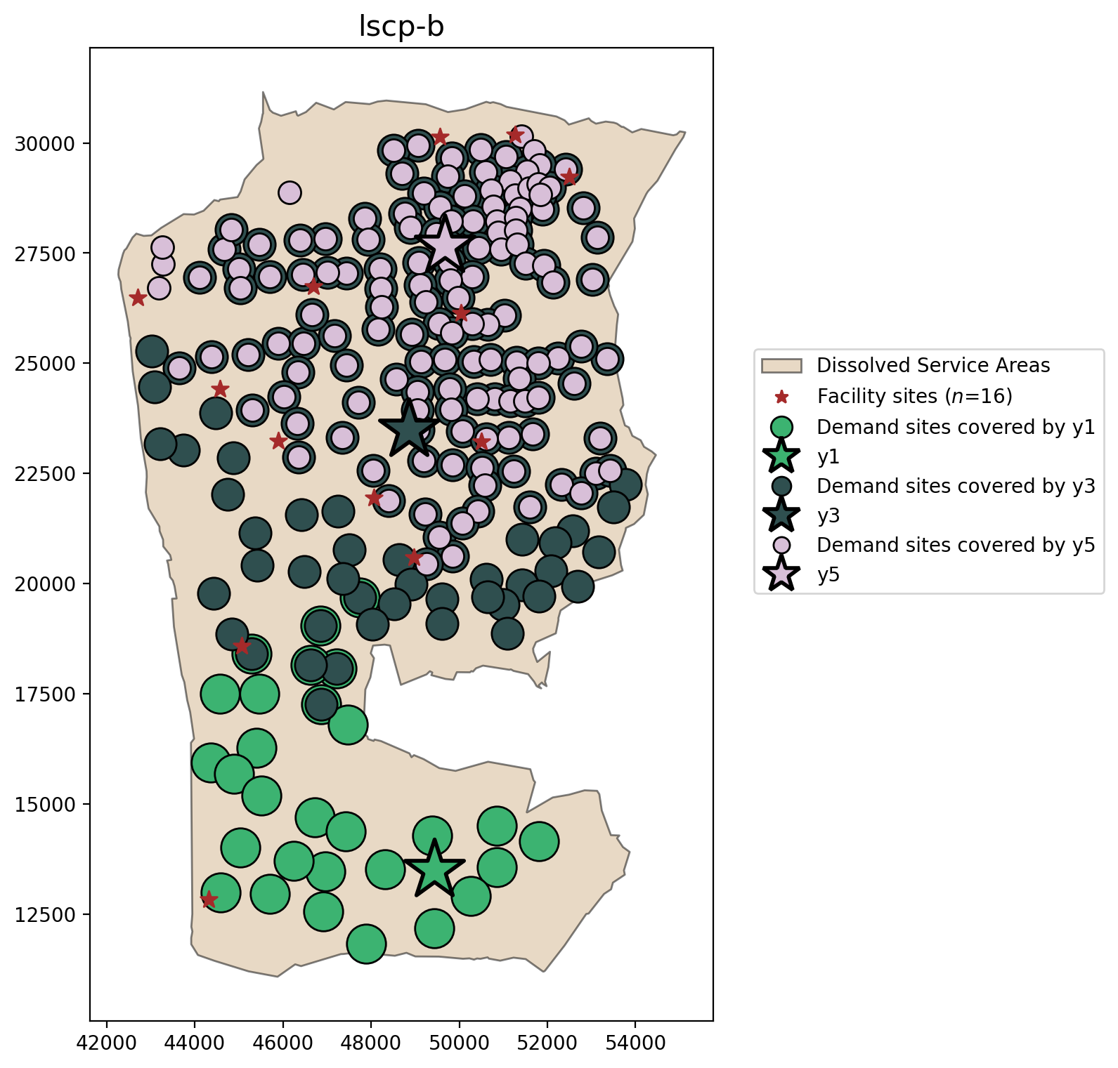
LSCP-B considering all candidate facilities
[29]:
plot_results(lscpb, lscpb.lscp_obj_value, facility_points, clis=demand_points)
[30]:
fig, axarr = plt.subplots(1, 2, figsize=(12, 6))
fig.subplots_adjust(wspace=-0.25)
for i, m in enumerate([lscp, lscpb]):
    _p = (
        m.lscp_obj_value if m.name.startswith("lscp-b") else m.problem.objective.value()
    )
    plot_results(m, _p, facility_points, clis=demand_points, ax=axarr[i])
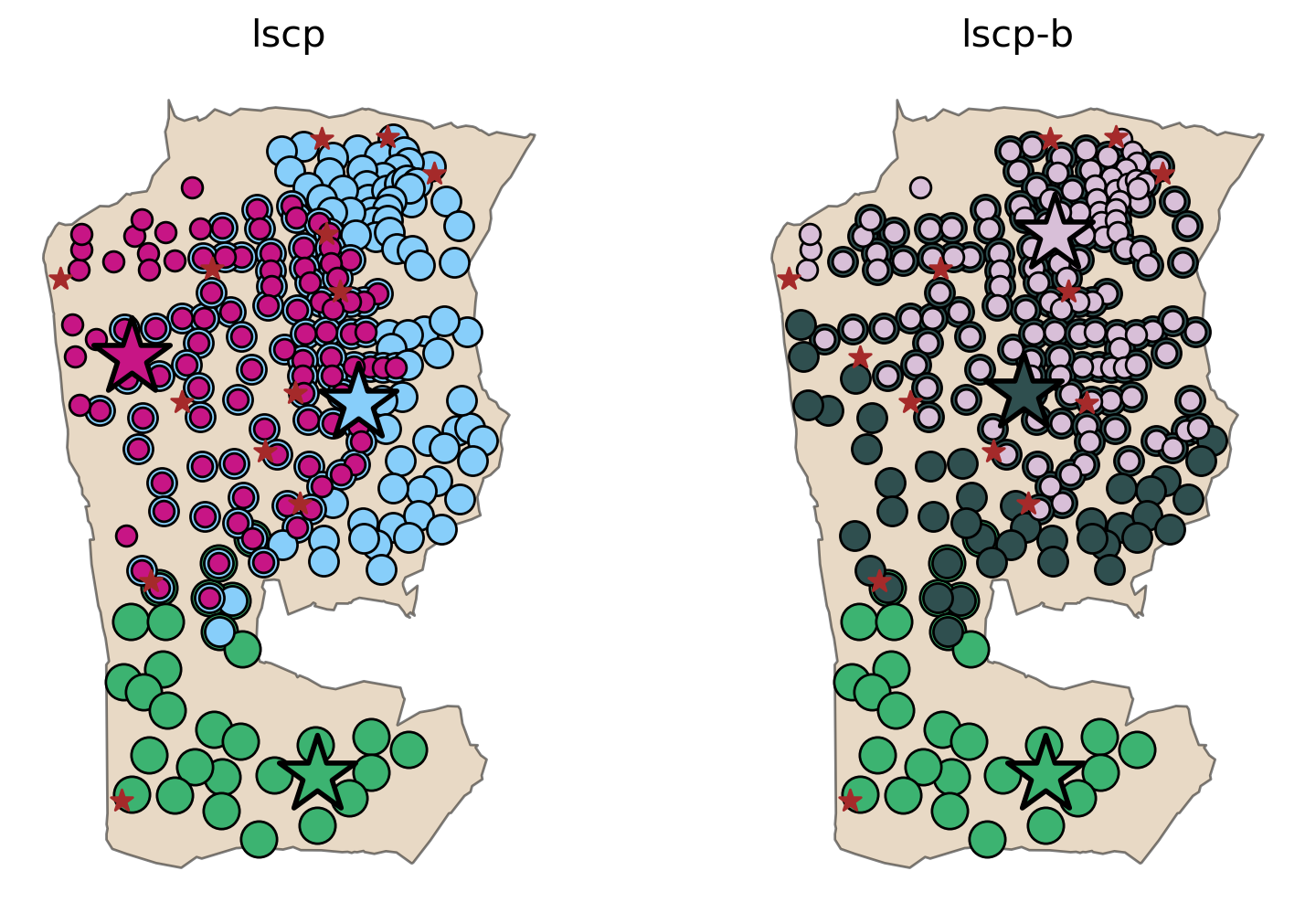
In both the LSCP and LSCP-B solutions facility \(y_1\) is included. However, \(y_4\) and \(y_{10}\) in the LSCP solution are swapped out for \(y_3\) and \(y_5\) in the LSCP-B solution to maximize backup coverage.
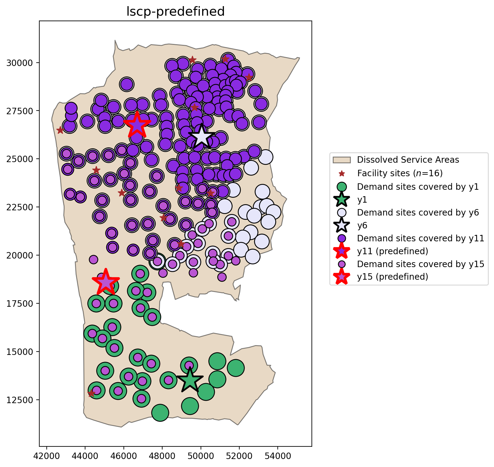
LSCP with selection of predefined candidate facilities
[31]:
plot_results(
    lscp_pre,
    lscp_pre.problem.objective.value(),
    facility_points,
    clis=demand_points,
)
LSCP-B with selection of predefined candidate facilities
[32]:
plot_results(lscpb_pre, lscpb_pre.lscp_obj_value, facility_points, clis=demand_points)
Comparing all models
[33]:
fig, axarr = plt.subplots(1, 2, figsize=(12, 6))
fig.subplots_adjust(wspace=-0.25)
for i, m in enumerate([lscp_pre, lscpb_pre]):
    _p = (
        m.lscp_obj_value if m.name.startswith("lscp-b") else m.problem.objective.value()
    )
    plot_results(m, _p, facility_points, clis=demand_points, ax=axarr[i])
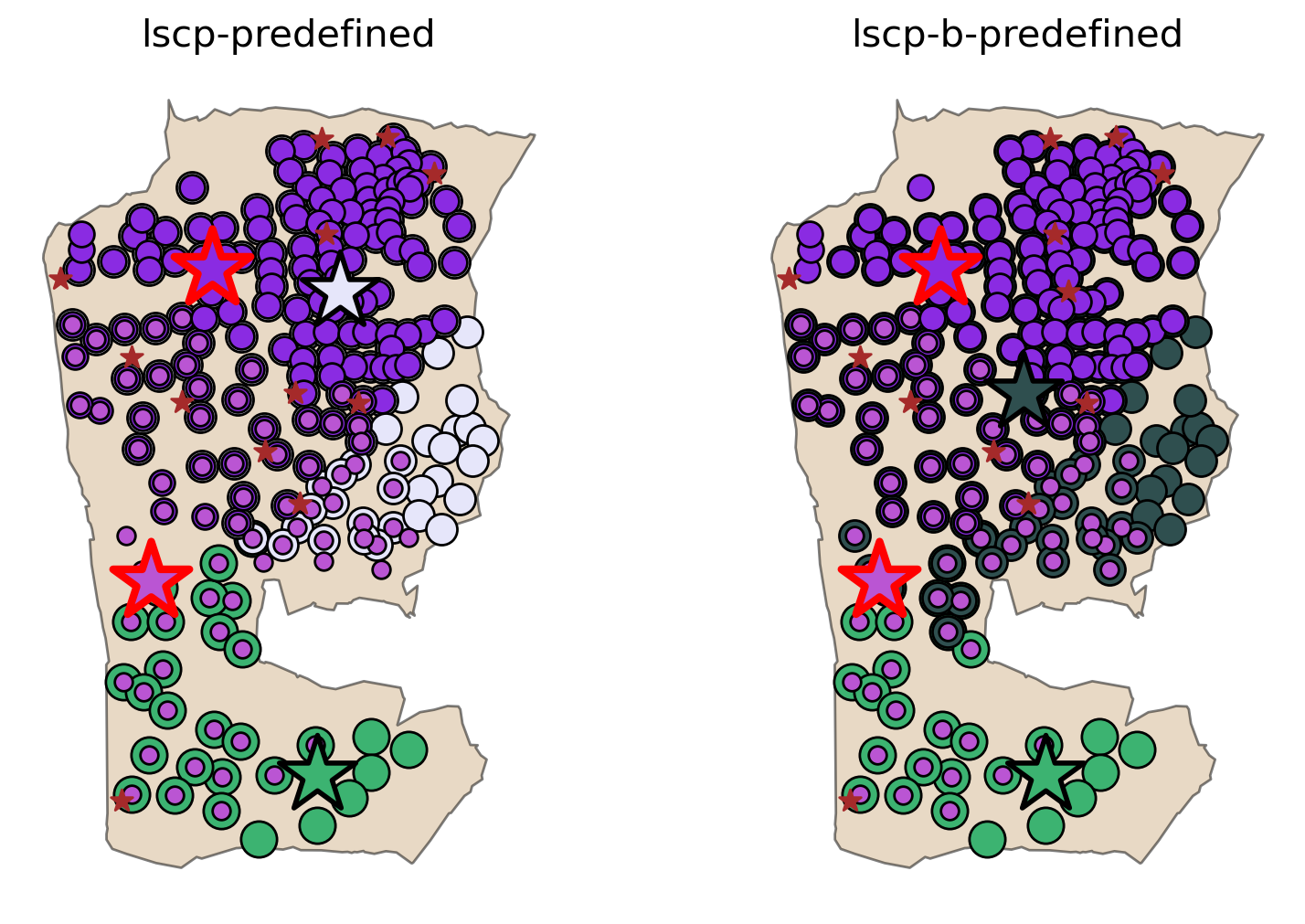
When stipulating that \(y_{11}\) and \(y_{15}\) must be included in the solution, the minimum number of facilities increases to 4, but as a result backup coverage also increases. Here we can see that facility \(y_1\) is again present in both solutions, where the LSCP opts for \(y_6\) and the LSCP-B opts for \(y_3\).
Evaluating available solvers
First we’ll determine which solvers are installed locally.
[34]:
with warnings.catch_warnings(record=True) as w:
    solvers = pulp.listSolvers(onlyAvailable=True)
for _w in w:
    print(_w.message)
solvers
[34]:
['GLPK_CMD', 'PULP_CBC_CMD', 'COIN_CMD', 'SCIP_CMD', 'HiGHS', 'HiGHS_CMD']
Above we can see that it returns a list with different solvers that are available. So, it’s up to the user to choose the best solver that fits the model. Let’s get the percentage as a metric to evaluate which solver is the best or improves the model.
[35]:
results = pandas.DataFrame(
    columns=["Solution Facilities", "Backup %", "Solve Time (sec.)"], index=solvers
)
for solver in solvers:
    _solver = pulp.getSolver(solver, msg=False)
    lscpb = LSCPB.from_cost_matrix(cost_matrix, SERVICE_RADIUS, _solver).solve()
    lscpb_perc = round(
        (lscpb.problem.objective.value() / len(lscpb.cli_vars)) * 100.0, 3
    )
    results.loc[solver] = [lscpb.lscp_obj_value, lscpb_perc, lscpb.problem.solutionTime]
results
Running HiGHS 1.10.0 (git hash: n/a): Copyright (c) 2025 HiGHS under MIT licence terms
MIP  has 205 rows; 16 cols; 1800 nonzeros; 16 integer variables (16 binary)
Coefficient ranges:
  Matrix [1e+00, 1e+00]
  Cost   [1e+00, 1e+00]
  Bound  [1e+00, 1e+00]
  RHS    [1e+00, 1e+00]
Presolving model
195 rows, 15 cols, 1760 nonzeros  0s
50 rows, 15 cols, 449 nonzeros  0s
50 rows, 6 cols, 234 nonzeros  0s
Objective function is integral with scale 1

Solving MIP model with:
   50 rows
   6 cols (6 binary, 0 integer, 0 implied int., 0 continuous)
   234 nonzeros

Src: B => Branching; C => Central rounding; F => Feasibility pump; H => Heuristic; L => Sub-MIP;
     P => Empty MIP; R => Randomized rounding; S => Solve LP; T => Evaluate node; U => Unbounded;
     z => Trivial zero; l => Trivial lower; u => Trivial upper; p => Trivial point; X => User solution

        Nodes      |    B&B Tree     |            Objective Bounds              |  Dynamic Constraints |       Work
Src  Proc. InQueue |  Leaves   Expl. | BestBound       BestSol              Gap |   Cuts   InLp Confl. | LpIters     Time

 u       0       0         0   0.00%   -inf            7                  Large        0      0      0         0     0.0s
 T       0       0         0 100.00%   2               3                 33.33%        0      0      0         3     0.0s
         1       0         1 100.00%   3               3                  0.00%        0      0      0         3     0.0s

Solving report
  Status            Optimal
  Primal bound      3
  Dual bound        3
  Gap               0% (tolerance: 0.01%)
  P-D integral      0.000123325386085
  Solution status   feasible
                    3 (objective)
                    0 (bound viol.)
                    0 (int. viol.)
                    0 (row viol.)
  Timing            0.00 (total)
                    0.00 (presolve)
                    0.00 (solve)
                    0.00 (postsolve)
  Max sub-MIP depth 0
  Nodes             1
  Repair LPs        0 (0 feasible; 0 iterations)
  LP iterations     3 (total)
                    0 (strong br.)
                    0 (separation)
                    0 (heuristics)
Running HiGHS 1.10.0 (git hash: n/a): Copyright (c) 2025 HiGHS under MIT licence terms
MIP  has 206 rows; 221 cols; 2018 nonzeros; 221 integer variables (221 binary)
Coefficient ranges:
  Matrix [1e+00, 1e+00]
  Cost   [1e+00, 1e+00]
  Bound  [1e+00, 1e+00]
  RHS    [1e+00, 3e+00]
Presolving model
203 rows, 217 cols, 1988 nonzeros  0s
203 rows, 217 cols, 1988 nonzeros  0s
Objective function is integral with scale 1

Solving MIP model with:
   203 rows
   217 cols (217 binary, 0 integer, 0 implied int., 0 continuous)
   1988 nonzeros

Src: B => Branching; C => Central rounding; F => Feasibility pump; H => Heuristic; L => Sub-MIP;
     P => Empty MIP; R => Randomized rounding; S => Solve LP; T => Evaluate node; U => Unbounded;
     z => Trivial zero; l => Trivial lower; u => Trivial upper; p => Trivial point; X => User solution

        Nodes      |    B&B Tree     |            Objective Bounds              |  Dynamic Constraints |       Work
Src  Proc. InQueue |  Leaves   Expl. | BestBound       BestSol              Gap |   Cuts   InLp Confl. | LpIters     Time

         0       0         0   0.00%   -205            inf                  inf        0      0      0         0     0.0s
 T       0       0         0   0.00%   -205            -143              43.36%        0      0      0       109     0.0s
         1       0         1 100.00%   -143            -143               0.00%        0      0      0       109     0.0s

Solving report
  Status            Optimal
  Primal bound      -143
  Dual bound        -143
  Gap               0% (tolerance: 0.01%)
  P-D integral      2.78219023811e-06
  Solution status   feasible
                    -143 (objective)
                    0 (bound viol.)
                    0 (int. viol.)
                    0 (row viol.)
  Timing            0.00 (total)
                    0.00 (presolve)
                    0.00 (solve)
                    0.00 (postsolve)
  Max sub-MIP depth 0
  Nodes             1
  Repair LPs        0 (0 feasible; 0 iterations)
  LP iterations     109 (total)
                    0 (strong br.)
                    0 (separation)
                    0 (heuristics)
[35]:
| Solution Facilities | Backup % | Solve Time (sec.) | |
|---|---|---|---|
| GLPK_CMD | 3 | 69.756 | 0.010166 |
| PULP_CBC_CMD | 3.0 | 69.756 | 0.023693 |
| COIN_CMD | 3.0 | 69.756 | 0.016525 |
| SCIP_CMD | 3.0 | 69.756 | 0.029387 |
| HiGHS | 3.0 | 69.756 | 0.004169 |
| HiGHS_CMD | 3.0 | 69.756 | 0.014144 |