This page was generated from notebooks/maxp.ipynb.
Interactive online version:
![]()
Max-P Regionalization
Authors: Sergio Rey, Xin Feng, James Gaboardi
The max-p problem involves the clustering of a set of geographic areas into the maximum number of homogeneous regions such that the value of a spatially extensive regional attribute is above a predefined threshold value. The spatially extensive attribute can be specified to ensure that each region contains sufficient population size, or a minimum number of enumeration units. The number of regions \(p\) is endogenous to the problem and is useful for regionalization problems where the
analyst does not require a fixed number of regions a-priori.
Originally formulated as a mixed-integer problem in Duque, Anselin, Rey (2012), max-p is an NP-hard problem and exact solutions are only feasible for small problem sizes. As such, a number of heuristic solution approaches have been suggested. PySAL implements the heuristic approach described in Wei, Rey, and Knaap
(2020).
[1]:
%config InlineBackend.figure_format = "retina"
%load_ext watermark
%watermark
Last updated: 2025-04-07T15:05:35.878470-04:00

Python implementation: CPython
Python version       : 3.12.9
IPython version      : 9.0.2

Compiler    : Clang 18.1.8
OS          : Darwin
Release     : 24.4.0
Machine     : arm64
Processor   : arm
CPU cores   : 8
Architecture: 64bit
[2]:
import warnings

import geopandas
import libpysal
import matplotlib.pyplot as plt
import numpy

import spopt
from spopt.region import MaxPHeuristic as MaxP

RANDOM_SEED = 123456

%watermark -w
%watermark -iv
Watermark: 2.5.0

spopt     : 0.6.2.dev3+g13ca45e
matplotlib: 3.10.1
libpysal  : 4.12.1
geopandas : 1.0.1
numpy     : 2.2.4
Mexican State Regional Income Clustering
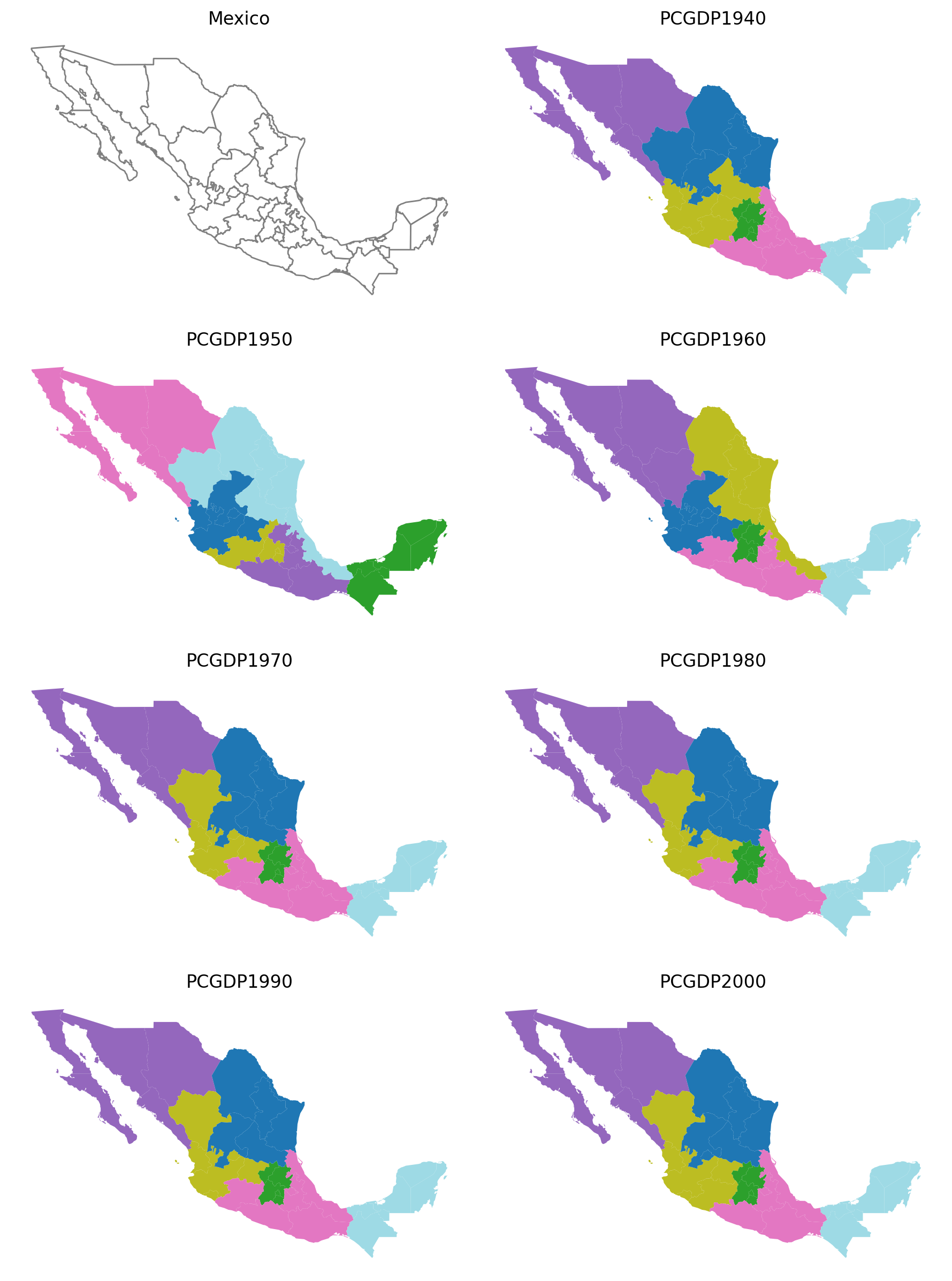
To illustrate maxp we utilize data on regional incomes for Mexican states over the period 1940-2000, originally used in Rey and Sastré-Gutiérrez (2010).
We can first explore the data by plotting the per capital gross regional domestic product (in constant USD 2000 dollars) for each year in the sample, using a quintile classification. Here we will define a function for creating subplots useful in visual comparisons, which also can solve Max-P instances and will be used again later).
[3]:
def subplotter(gdf, incrs, w, threshold=5, top_n=2, seed=RANDOM_SEED):
    """Helper plotting function, also solves MaxP instances if desired."""
    rows, cols = incrs.shape
    f, axs = plt.subplots(rows, cols, figsize=(9, 14))
    for i in range(rows):
        for j in range(cols):
            year, _ax = incrs[i, j], axs[i, j]
            if not year:
                # plot country geographies
                _attr = "Mexico"
                gdf.plot(ax=_ax, ec="grey", fc="white")
            else:
                _attr = f"PCGDP{year}"
                if not w:
                    # plot country geographies by attributes
                    plt_kws = {"scheme": "Quantiles", "cmap": "GnBu", "ec": "grey"}
                    plt_kws.update({"legend_kwds": {"fmt": "{:.0f}"}})
                    gdf.plot(column=_attr, ax=_ax, legend=True, **plt_kws)
                else:
                    # solve a MaxP instance and plot regions
                    numpy.random.seed(seed)
                    maxp_args = gdf, w, _attr, "count", threshold
                    model = MaxP(*maxp_args, top_n=top_n)
                    model.solve()
                    label = year + "labels_"
                    gdf[label] = model.labels_
                    gdf.plot(column=label, ax=_ax, cmap="tab20")
            _ax.set_title(_attr)
            _ax.set_axis_off()
            _ax.set_aspect("equal")
    f.subplots_adjust(wspace=-0.7, hspace=-0.65)
    f.tight_layout()
[4]:
pth = libpysal.examples.get_path("mexicojoin.shp")
mexico = geopandas.read_file(pth)
mexico.head()
[4]:
| POLY_ID | AREA | CODE | NAME | PERIMETER | ACRES | HECTARES | PCGDP1940 | PCGDP1950 | PCGDP1960 | ... | GR9000 | LPCGDP40 | LPCGDP50 | LPCGDP60 | LPCGDP70 | LPCGDP80 | LPCGDP90 | LPCGDP00 | TEST | geometry | |
|---|---|---|---|---|---|---|---|---|---|---|---|---|---|---|---|---|---|---|---|---|---|
| 0 | 1 | 7.252751e+10 | MX02 | Baja California Norte | 2040312.385 | 1.792187e+07 | 7252751.376 | 22361.0 | 20977.0 | 17865.0 | ... | 0.05 | 4.35 | 4.32 | 4.25 | 4.40 | 4.47 | 4.43 | 4.48 | 1.0 | MULTIPOLYGON (((-113.13972 29.01778, -113.2405... |
| 1 | 2 | 7.225988e+10 | MX03 | Baja California Sur | 2912880.772 | 1.785573e+07 | 7225987.769 | 9573.0 | 16013.0 | 16707.0 | ... | 0.00 | 3.98 | 4.20 | 4.22 | 4.39 | 4.46 | 4.41 | 4.42 | 2.0 | MULTIPOLYGON (((-111.20612 25.80278, -111.2302... |
| 2 | 3 | 2.731957e+10 | MX18 | Nayarit | 1034770.341 | 6.750785e+06 | 2731956.859 | 4836.0 | 7515.0 | 7621.0 | ... | -0.05 | 3.68 | 3.88 | 3.88 | 4.04 | 4.13 | 4.11 | 4.06 | 3.0 | MULTIPOLYGON (((-106.62108 21.56531, -106.6475... |
| 3 | 4 | 7.961008e+10 | MX14 | Jalisco | 2324727.436 | 1.967200e+07 | 7961008.285 | 5309.0 | 8232.0 | 9953.0 | ... | 0.03 | 3.73 | 3.92 | 4.00 | 4.21 | 4.32 | 4.30 | 4.33 | 4.0 | POLYGON ((-101.5249 21.85664, -101.5883 21.772... |
| 4 | 5 | 5.467030e+09 | MX01 | Aguascalientes | 313895.530 | 1.350927e+06 | 546702.985 | 10384.0 | 6234.0 | 8714.0 | ... | 0.13 | 4.02 | 3.79 | 3.94 | 4.21 | 4.32 | 4.32 | 4.44 | 5.0 | POLYGON ((-101.8462 22.01176, -101.9653 21.883... |
5 rows × 35 columns
[5]:
mxgdp_years = [str(x) for x in range(1940, 2010, 10)]
mxgdp_years = numpy.array([None] + mxgdp_years)
mxgdp_years_grid = mxgdp_years.reshape(4, 2)
mxgdp_years_grid
[5]:
array([[None, '1940'],
       ['1950', '1960'],
       ['1970', '1980'],
       ['1990', '2000']], dtype=object)
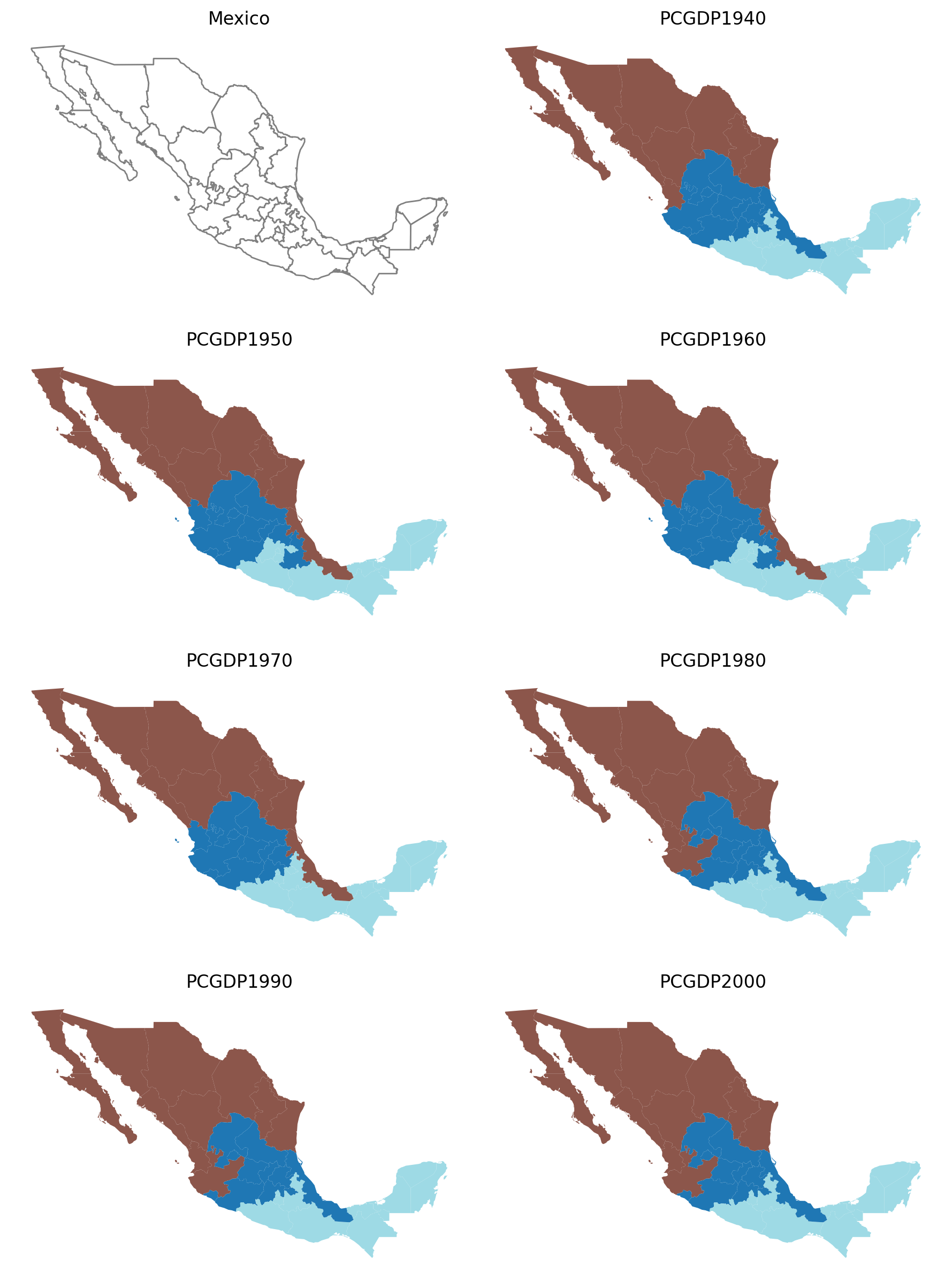
Regional incomes for Mexican states over the period 1940-2000
[6]:
subplotter(mexico, mxgdp_years_grid, None)
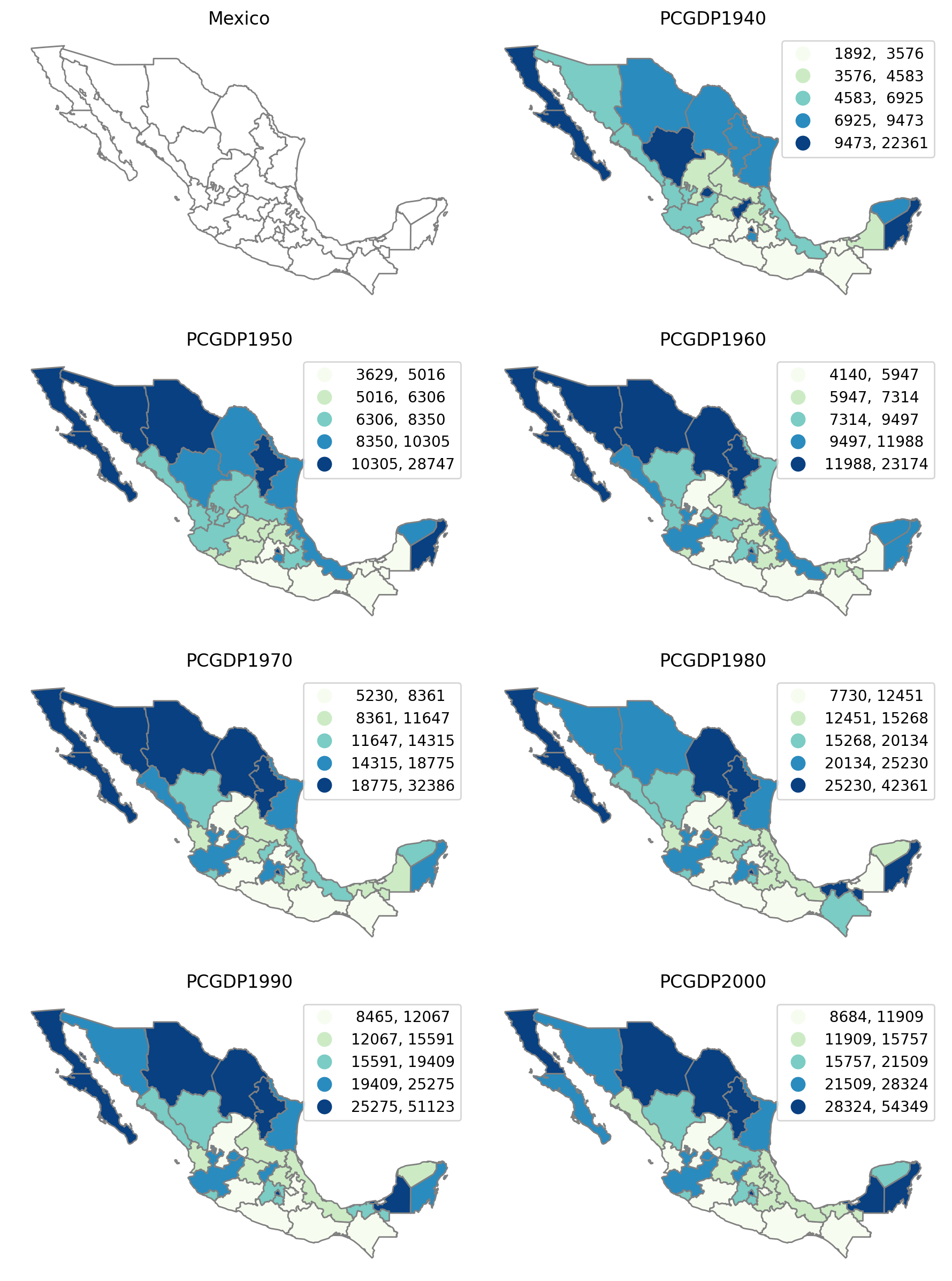
In general terms, the north-south divide in incomes is present in each of the 7 decades. There is some variation in states moving across quintiles however, and this is true at both the bottom and top of the state income distribution.
To develop a holistic view of the Mexican space economy over this timespan, we can try to form a set of spatially connected regions that maximizes the internal socieconomic levels of the states belonging to each region.
Pooled Regionalization
To develop our holistic view, we can treat the six cross-sections as a multidimensional array and seek to cluster 32 Mexican states into the maximum number of regions such that each region as at least 6 = 32 // 5 states and homogeneity in per capita gross regional product over 1940-2000 is maximized.
We first define the variables in the dataframe that will be used to measure regional homogeneity:
[7]:
attrs_name = [f"PCGDP{year}" for year in mxgdp_years[1:]]
attrs_name
[7]:
['PCGDP1940',
 'PCGDP1950',
 'PCGDP1960',
 'PCGDP1970',
 'PCGDP1980',
 'PCGDP1990',
 'PCGDP2000']
Next, we specify a number of parameters that will serve as input to the max-p model.
A spatial weights object expresses the spatial connectivity of the states:
[8]:
with warnings.catch_warnings(record=True):
    w = libpysal.weights.Queen.from_dataframe(mexico)
The remaining arguments are the minimum number of states each region must have (threshold):
[9]:
threshold = 6
and the number of the top candidate regions to consider when assigning enclaves (top_n):
[10]:
top_n = 2
We create the attribute count which will serve as the threshold attribute which we add to the dataframe:
[11]:
mexico["count"] = 1
threshold_name = "count"
The model can then be instantiated and solved:
[12]:
numpy.random.seed(RANDOM_SEED)
model = MaxP(mexico, w, attrs_name, threshold_name, threshold, top_n)
model.solve()
[13]:
mexico["maxp_new"] = model.labels_
[14]:
mexico[["maxp_new", "AREA"]].groupby(by="maxp_new").count()
[14]:
| AREA | |
|---|---|
| maxp_new | |
| 1 | 6 |
| 2 | 7 |
| 3 | 6 |
| 4 | 7 |
| 5 | 6 |
[15]:
model.p
[15]:
5
[16]:
mexico.plot(figsize=(8, 5), column="maxp_new", cmap="tab20", edgecolor="w").axis("off");
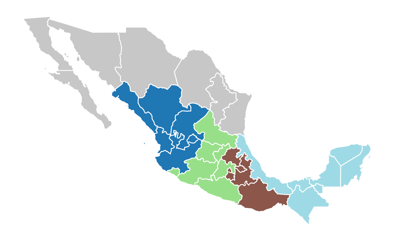
The model solution results in five regions, three of which have six states, and two with seven states each. Each region is a spatially connected component, as required by the max-p problem.
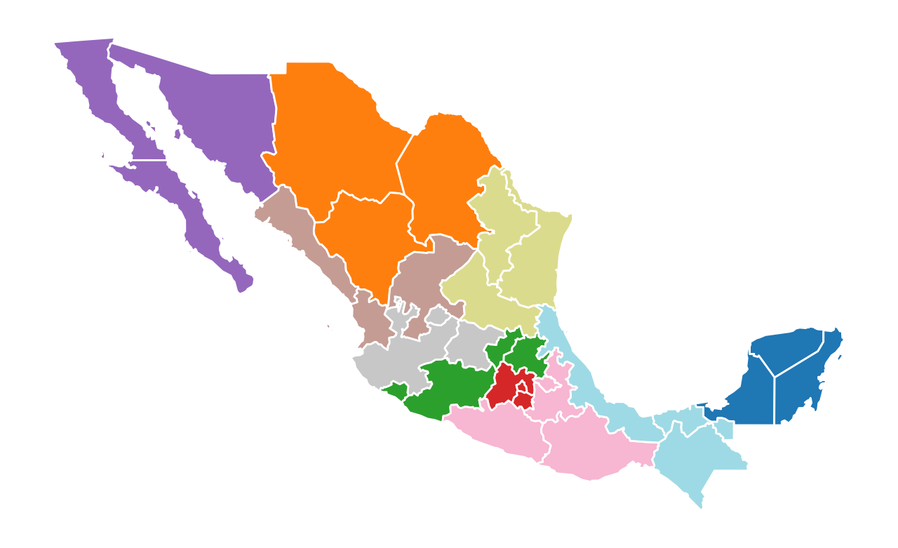
Change threshold to a minimum of 3 states per region
[17]:
numpy.random.seed(RANDOM_SEED)
threshold = 3
model = MaxP(mexico, w, attrs_name, threshold_name, threshold, top_n)
model.solve()
[18]:
mexico["maxp_3"] = model.labels_
mexico[["maxp_3", "AREA"]].groupby(by="maxp_3").count()
[18]:
| AREA | |
|---|---|
| maxp_3 | |
| 1 | 3 |
| 2 | 3 |
| 3 | 4 |
| 4 | 3 |
| 5 | 3 |
| 6 | 3 |
| 7 | 4 |
| 8 | 3 |
| 9 | 3 |
| 10 | 3 |
[19]:
model.p
[19]:
10
[20]:
mexico.plot(figsize=(8, 5), column="maxp_3", cmap="tab20", edgecolor="w").axis("off");
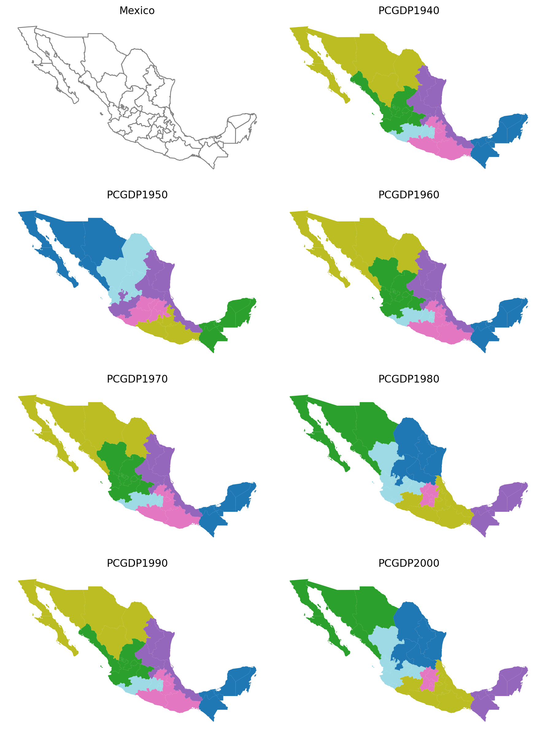
Year-by-Year Regionalization while Varying Parameters
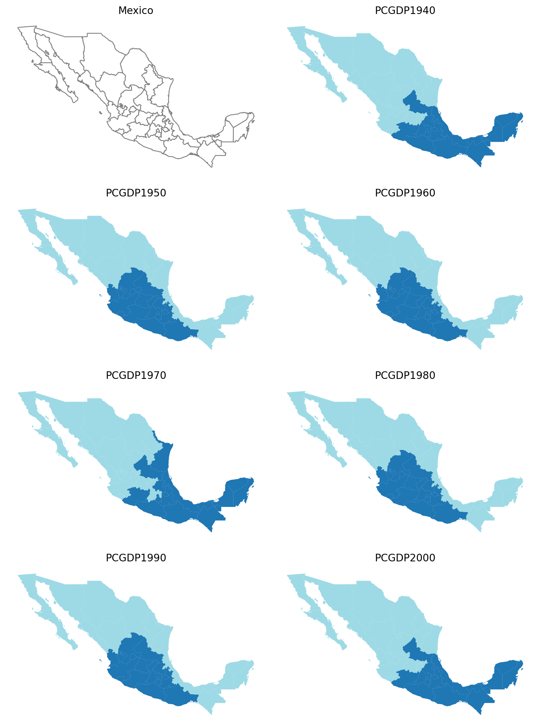
Vary minimum in-region threshold (5, 10, 15); hold enclave assignment constant (2)
5 states
[21]:
region_args = mexico, mxgdp_years_grid, w
[22]:
subplotter(*region_args, threshold=5, top_n=2)
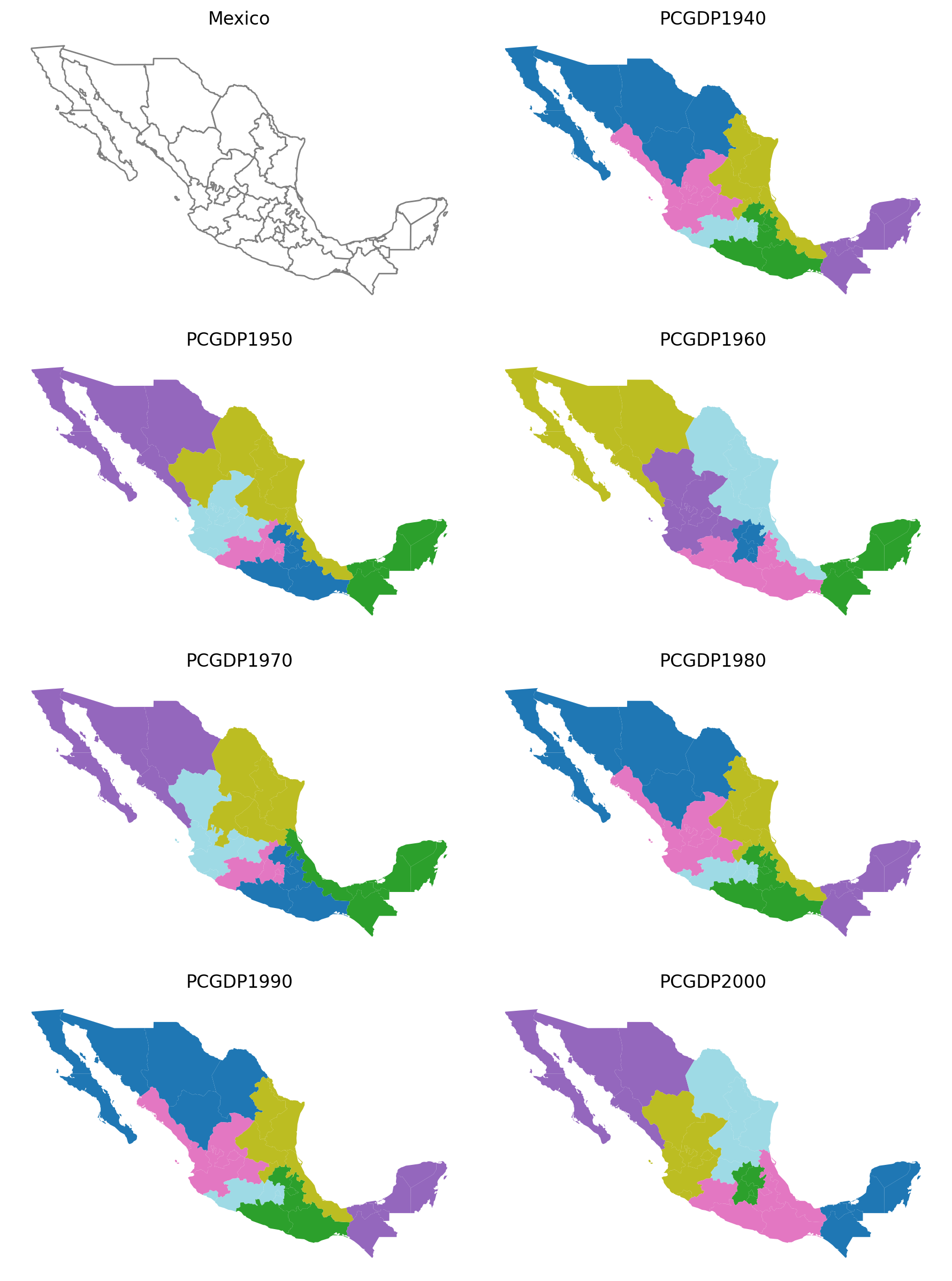
10 states
[23]:
subplotter(*region_args, threshold=10, top_n=2)
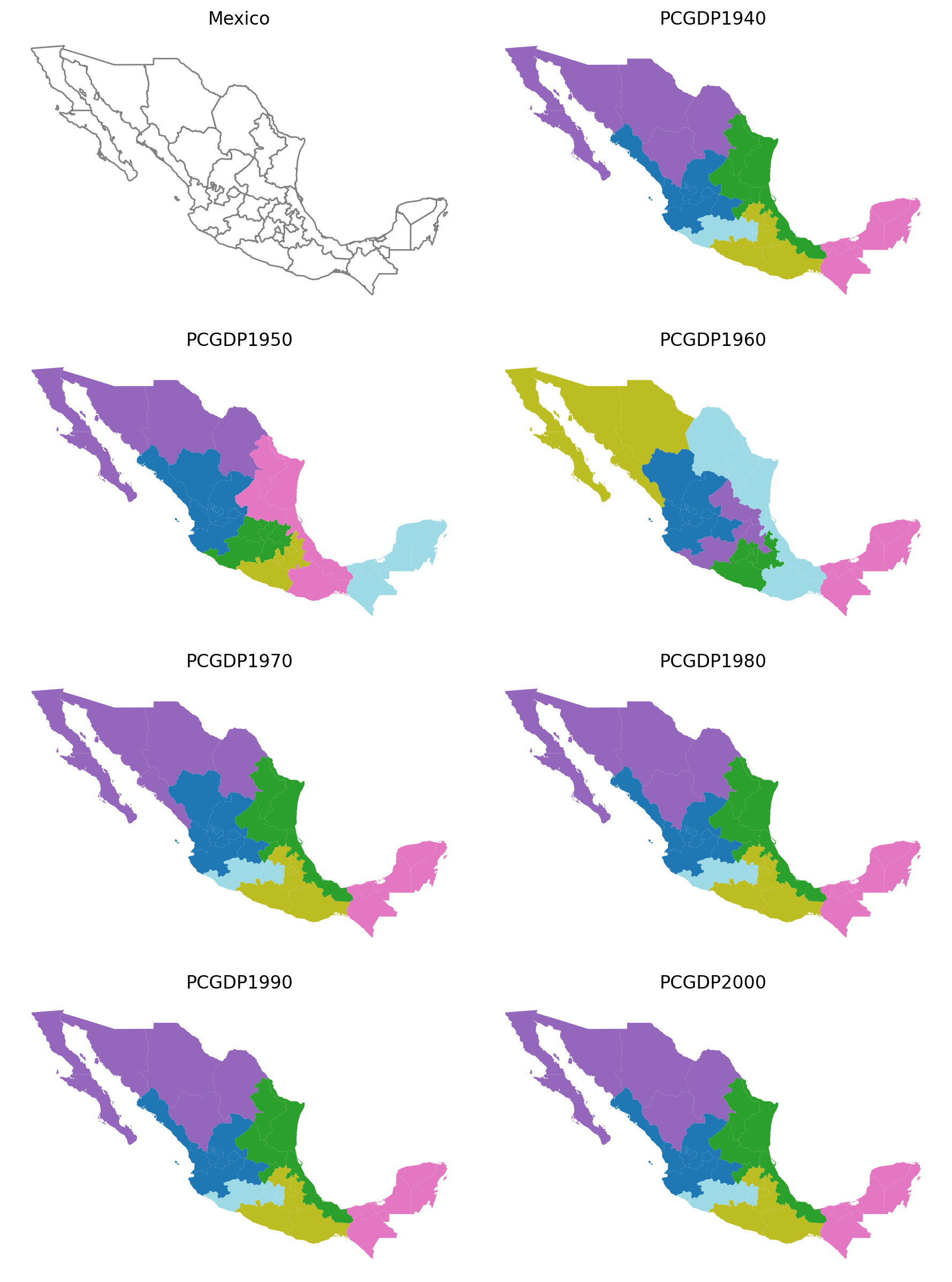
15 states
[24]:
subplotter(*region_args, threshold=15, top_n=2)
Vary state enclave assignments (1, 3, 5); hold minimum in-region threshold constant (5)
1 state
[25]:
subplotter(*region_args, threshold=5, top_n=1)
3 states
[26]:
subplotter(*region_args, threshold=5, top_n=3)
5 states
[27]:
subplotter(*region_args, threshold=5, top_n=5)
As shown here, varying the threshold and top_n parameters both have a demonstrable effect regionalization outcomes.