This page was generated from notebooks/transportation-problem.ipynb.
Interactive online version:
![]()
If any part of this notebook is used in your research, please cite with the reference found in README.md.
The Transportation Problem
Integrating pysal/spaghetti and python-mip for optimal shipping
Author: James D. Gaboardi jgaboardi@gmail.com
This notebook provides a use case for:
Introducing the Transportation Problem
Declaration of a solution class and model parameters
Solving the Transportation Problem for an optimal shipment plan
[1]:
%config InlineBackend.figure_format = "retina"
[2]:
%load_ext watermark
%watermark
Last updated: 2022-11-01T23:22:10.592678-04:00

Python implementation: CPython
Python version       : 3.10.6
IPython version      : 8.6.0

Compiler    : Clang 13.0.1
OS          : Darwin
Release     : 22.1.0
Machine     : x86_64
Processor   : i386
CPU cores   : 8
Architecture: 64bit
[3]:
import geopandas
from libpysal import examples
import matplotlib
import mip
import numpy
import os
import spaghetti
import matplotlib_scalebar
from matplotlib_scalebar.scalebar import ScaleBar

%matplotlib inline
%watermark -w
%watermark -iv
Watermark: 2.3.1

numpy              : 1.23.4
mip                : 1.14.1
libpysal           : 4.6.2
matplotlib         : 3.6.1
spaghetti          : 1.6.8
geopandas          : 0.12.1
json               : 2.0.9
matplotlib_scalebar: 0.8.0
/Users/the-gaboardi/miniconda3/envs/py310_spgh_dev/lib/python3.10/site-packages/spaghetti/network.py:39: FutureWarning: The next major release of pysal/spaghetti (2.0.0) will drop support for all ``libpysal.cg`` geometries. This change is a first step in refactoring ``spaghetti`` that is expected to result in dramatically reduced runtimes for network instantiation and operations. Users currently requiring network and point pattern input as ``libpysal.cg`` geometries should prepare for this simply by converting to ``shapely`` geometries.
  warnings.warn(f"{dep_msg}", FutureWarning)
1 Introduction
Scenario
There are 8 schools in Neighborhood Y of City X and a total of 100 microscopes for the biology classes at the 8 schools, though the microscopes are not evenly distributed across the locations. Since last academic year there has been a significant enrollment shift in the neighborhood, and at 4 of the schools there is a surplus whereas the remaining 4 schools require additional microscopes. Dr. Rachel Carson, the head of the biology department at City X’s School Board decides to utilize a mathematical programming model to solve the microscope discrepency. After consideration, she selects the Transportation Problem.
The Transportation Problem seeks to allocate supply to demand while minimizing transportation costs and was formally described by Hitchcock (1941). Supply (\(\textit{n}\)) and demand (\(\textit{m}\)) are generally represented as unit weights of decision variables at facilities along a network with the time or distance between nodes representing the cost of transporting one unit from a supply node to a demand node. These costs are stored in an \(\textit{n x m}\) cost matrix.
Integer Linear Programming Formulation based on Daskin (2013, Ch. 2).
:math:`begin{array} displaystyle normalsize textrm{Minimize} & displaystyle normalsize sum_{i in I} sum_{j in J} c_{ij}x_{ij} & & & & normalsize (1) \ normalsize textrm{Subject To} & displaystyle normalsize sum_{j in J} x_{ij} leq S_i & normalsize forall i in I; & & &normalsize (2)\
& displaystyle normalsize sum_{i in I} x_{ij} geq D_j & normalsize forall j in J; & & &normalsize (3)\
& displaystyle normalsize x_{ij} geq 0 & displaystyle normalsize forall i in I & displaystyle normalsize normalsize forall j in j. & &normalsize (4)\ end{array}`
\(\begin{array} \displaystyle \normalsize \textrm{Where} & \small i & \small = & \small \textrm{each potential origin node} &&&&\\ & \small I & \small = & \small \textrm{the complete set of potential origin nodes} &&&&\\ & \small j & \small = & \small \textrm{each potential destination node} &&&&\\ & \small J & \small = & \small \textrm{the complete set of potential destination nodes} &&&&\\ & \small x_{ij} & \small = & \small \textrm{amount to be shipped from } i \in I \textrm{ to } j \in J &&&&\\ & \small c_{ij} & \small = & \small \textrm{per unit shipping costs between all } i,j \textrm{ pairs} &&&& \\ & \small S_i & \small = & \small \textrm{node } i \textrm{ supply for } i \in I &&&&\\ & \small D_j & \small = & \small \textrm{node } j \textrm{ demand for } j \in J &&&&\\ \end{array}\)
References
Church, Richard L. and Murray, Alan T. (2009) Business Site Selection, Locational Analysis, and GIS. Hoboken. John Wiley & Sons, Inc.
Daskin, M. (2013) Network and Discrete Location: Models, Algorithms, and Applications. New York: John Wiley & Sons, Inc.
Gass, S. I. and Assad, A. A. (2005) An Annotated Timeline of Operations Research: An Informal History. Springer US.
Hitchcock, Frank L. (1941) The Distribution of a Product from Several Sources to Numerous Localities. Journal of Mathematics and Physics. 20(1):224-230.
Koopmans, Tjalling C. (1949) Optimum Utilization of the Transportation System. Econometrica. 17:136-146.
Miller, H. J. and Shaw, S.-L. (2001) Geographic Information Systems for Transportation: Principles and Applications. New York. Oxford University Press.
Phillips, Don T. and Garcia‐Diaz, Alberto. (1981) Fundamentals of Network Analysis. Englewood Cliffs. Prentice Hall.
2. A model, data, and parameters
Schools labeled as either ‘supply’ or ‘demand’ locations
[4]:
supply_schools = [1, 6, 7, 8]
demand_schools = [2, 3, 4, 5]
Amount of supply and demand at each location (indexed by supply_schools and demand_schools)
[5]:
amount_supply = [20, 30, 15, 35]
amount_demand = [5, 45, 10, 40]
Solution class
[6]:
class TransportationProblem:
    def __init__(
        self,
        supply_nodes,
        demand_nodes,
        cij,
        si,
        dj,
        xij_tag="x_%s,%s",
        supply_constr_tag="supply(%s)",
        demand_constr_tag="demand(%s)",
        solver="cbc",
        display=True,
    ):
        """Instantiate and solve the Primal Transportation Problem
        based the formulation from Daskin (2013, Ch. 2).

        Parameters
        ----------
        supply_nodes : geopandas.GeoSeries
            Supply node decision variables.
        demand_nodes : geopandas.GeoSeries
            Demand node decision variables.
        cij : numpy.array
            Supply-to-demand distance matrix for nodes.
        si : geopandas.GeoSeries
            Amount that can be supplied by each supply node.
        dj : geopandas.GeoSeries
            Amount that can be received by each demand node.
        xij_tag : str
            Shipping decision variable names within the model. Default is
            'x_%s,%s' where %s indicates string formatting.
        supply_constr_tag : str
            Supply constraint labels. Default is 'supply(%s)'.
        demand_constr_tag : str
            Demand constraint labels. Default is 'demand(%s)'.
        solver : str
            Default is 'cbc' (coin-branch-cut). Can be set
            to 'gurobi' (if Gurobi is installed).
        display : bool
            Print out solution results.

        Attributes
        ----------
        supply_nodes : See description in above.
        demand_nodes : See description in above.
        cij : See description in above.
        si : See description in above.
        dj : See description in above.
        xij_tag : See description in above.
        supply_constr_tag : See description in above.
        demand_constr_tag : See description in above.
        rows : int
            The number of supply nodes.
        rrows : range
            The index of supply nodes.
        cols : int
            The number of demand nodes.
        rcols : range
            The index of demand nodes.
        model : mip.model.Model
            Integer Linear Programming problem instance.
        xij : numpy.array
            Shipping decision variables (``mip.entities.Var``).
        """

        # all nodes to be visited
        self.supply_nodes, self.demand_nodes = supply_nodes, demand_nodes
        # shipping costs (distance matrix) and amounts
        self.cij, self.si, self.dj = cij, si.values, dj.values
        self.ensure_float()
        # alpha tag for decision variables
        self.xij_tag = xij_tag
        # alpha tag for supply and demand constraints
        self.supply_constr_tag = supply_constr_tag
        self.demand_constr_tag = demand_constr_tag

        # instantiate a model
        self.model = mip.Model(" TransportationProblem", solver_name=solver)
        # define row and column indices
        self.rows, self.cols = self.si.shape[0], self.dj.shape[0]
        self.rrows, self.rcols = range(self.rows), range(self.cols)
        # create and set the decision variables
        self.shipping_dvs()
        # set the objective function
        self.objective_func()
        # add supply constraints
        self.add_supply_constrs()
        # add demand constraints
        self.add_demand_constrs()
        # solve
        self.solve(display=display)
        # shipping decisions lookup
        self.get_decisions(display=display)

    def ensure_float(self):
        """Convert integers to floats (rough edge in mip.LinExpr)"""
        self.cij = self.cij.astype(float)
        self.si = self.si.astype(float)
        self.dj = self.dj.astype(float)

    def shipping_dvs(self):
        """Create the shipping decision variables - eq (4)."""

        def _s(_x):
            """Helper for naming variables"""
            return self.supply_nodes[_x].split("_")[-1]

        def _d(_x):
            """Helper for naming variables"""
            return self.demand_nodes[_x].split("_")[-1]

        xij = numpy.array(
            [
                [self.model.add_var(self.xij_tag % (_s(i), _d(j))) for j in self.rcols]
                for i in self.rrows
            ]
        )
        self.xij = xij

    def objective_func(self):
        """Add the objective function - eq (1)."""
        self.model.objective = mip.minimize(
            mip.xsum(
                self.cij[i, j] * self.xij[i, j] for i in self.rrows for j in self.rcols
            )
        )

    def add_supply_constrs(self):
        """Add supply contraints to the model - eq (2)."""
        for i in self.rrows:
            rhs, label = self.si[i], self.supply_constr_tag % i
            self.model += mip.xsum(self.xij[i, j] for j in self.rcols) <= rhs, label

    def add_demand_constrs(self):
        """Add demand contraints to the model - eq (3)."""
        for j in self.rcols:
            rhs, label = self.dj[j], self.demand_constr_tag % j
            self.model += mip.xsum(self.xij[i, j] for i in self.rrows) >= rhs, label

    def solve(self, display=True):
        """Solve the model"""
        self.model.optimize()
        if display:
            obj = round(self.model.objective_value, 4)
            print("Minimized shipping costs: %s" % obj)

    def get_decisions(self, display=True):
        """Fetch the selected decision variables."""
        shipping_decisions = {}
        if display:
            print("\nShipping decisions:")
        for i in self.rrows:
            for j in self.rcols:
                v, vx = self.xij[i, j], self.xij[i, j].x
                if vx > 0:
                    if display:
                        print("\t", v, vx)
                    shipping_decisions[v.name] = vx
        self.shipping_decisions = shipping_decisions

    def print_lp(self, name=None):
        """Save LP file in order to read in and print."""
        if not name:
            name = self.model.name
        lp_file_name = "%s.lp" % name
        self.model.write(lp_file_name)
        lp_file = open(lp_file_name, "r")
        lp = lp_file.read()
        print("\n", lp)
        lp_file.close()
        os.remove(lp_file_name)

    def extract_shipments(self, paths, id_col, ship="ship"):
        """Extract the supply to demand shipments as a
        ``geopandas.GeoDataFrame`` of ``shapely.geometry.LineString`` objects.

        Parameters
        ----------
        paths : geopandas.GeoDataFrame
            Shortest-path routes between all ``self.supply_nodes``
            and ``self.demand_nodes``.
        id_col : str
            ID column name.
        ship : str
            Column name for the amount of good shipped.
            Default is 'ship'.

        Returns
        -------
        shipments : geopandas.GeoDataFrame
            Optimal shipments from ``self.supply_nodes`` to
            ``self.demand_nodes``.
        """

        def _id(sp):
            """ID label helper"""
            return tuple([int(i) for i in sp.split("_")[-1].split(",")])

        paths[ship] = int
        # set label of the shipping path for each OD pair.
        for ship_path, shipment in self.shipping_decisions.items():
            paths.loc[(paths[id_col] == _id(ship_path)), ship] = shipment
        # extract only shiiping paths
        shipments = paths[paths[ship] != int].copy()
        shipments[ship] = shipments[ship].astype(int)

        return shipments
Plotting helper functions and constants
Note: originating shipments
[7]:
shipping_colors = ["maroon", "cyan", "magenta", "orange"]
[8]:
def obs_labels(o, b, s, col="id", **kwargs):
    """Label each point pattern observation."""

    def _lab_loc(_x):
        """Helper for labeling observations."""
        return _x.geometry.coords[0]

    if o.index.name != "schools":
        X = o.index.name[0]
    else:
        X = ""
    kws = {"size": s, "ha": "left", "va": "bottom", "style": "oblique"}
    kws.update(kwargs)
    o.apply(lambda x: b.annotate(text=X+str(x[col]), xy=_lab_loc(x), **kws), axis=1)
[9]:
def make_patches(objects):
    """Create patches for legend"""
    patches = []
    for _object in objects:
        try:
            oname = _object.index.name
        except AttributeError:
            oname = "shipping"
        if oname.split(" ")[0] in ["schools", "supply", "demand"]:
            ovalue = _object.shape[0]
            if oname == "schools":
                ms, m, c, a = 3, "o", "k", 1
            elif oname.startswith("supply"):
                ms, m, c, a = 10, "o", "b", 0.25
            elif oname.startswith("demand"):
                ms, m, c, a = 10, "o", "g", 0.25
            if oname.endswith("snapped"):
                ms, m, a = float(ms) / 2.0, "x", 1
            _kws = {"lw": 0, "c": c, "marker": m, "ms": ms, "alpha": a}
            label = "%s — %s" % (oname.capitalize(), int(ovalue))
            p = matplotlib.lines.Line2D([], [], label=label, **_kws)
            patches.append(p)
        else:
            patch_info = plot_shipments(_object, "", for_legend=True)
            for c, lw, lwsc, (i, j) in patch_info:
                label = "s%s$\\rightarrow$d%s — %s microscopes" % (i, j, lw)
                _kws = {"alpha": 0.75, "c": c, "lw": lwsc, "label": label}
                p = matplotlib.lines.Line2D([], [], solid_capstyle="round", **_kws)
                patches.append(p)
    return patches
[10]:
def legend(objects, anchor=(1.005, 1.016)):
    """Add a legend to a plot"""
    patches = make_patches(objects)
    kws = {"fancybox": True, "framealpha": 0.85, "fontsize": "x-large"}
    kws.update({"bbox_to_anchor":anchor, "labelspacing":2., "borderpad":2.})
    legend = matplotlib.pyplot.legend(handles=patches, **kws)
    legend.get_frame().set_facecolor("white")
[11]:
def plot_shipments(sd, b, scaled=0.75, for_legend=False):
    """Helper for plotting shipments based on OD and magnitude"""
    _patches = []
    _plot_kws = {"alpha":0.75, "zorder":0, "capstyle":"round"}
    for c, (g, gdf) in zip(shipping_colors, sd):
        lw, lw_scaled, ids = gdf["ship"], gdf["ship"] * scaled, gdf["id"]
        if for_legend:
            for _lw, _lwsc, _id in zip(lw, lw_scaled, ids):
                _patches.append([c, _lw, _lwsc, _id])
        else:
            gdf.plot(ax=b, color=c, lw=lw_scaled, **_plot_kws)
    if for_legend:
        return _patches
Streets
[12]:
streets = geopandas.read_file(examples.get_path("streets.shp"))
streets.crs = "esri:102649"
streets = streets.to_crs("epsg:2762")
Schools
[13]:
schools = geopandas.read_file(examples.get_path("schools.shp"))
schools.index.name = "schools"
schools.crs = "esri:102649"
schools = schools.to_crs("epsg:2762")
Schools - supply nodes
[14]:
schools_supply = schools[schools["POLYID"].isin(supply_schools)]
schools_supply.index.name = "supply"
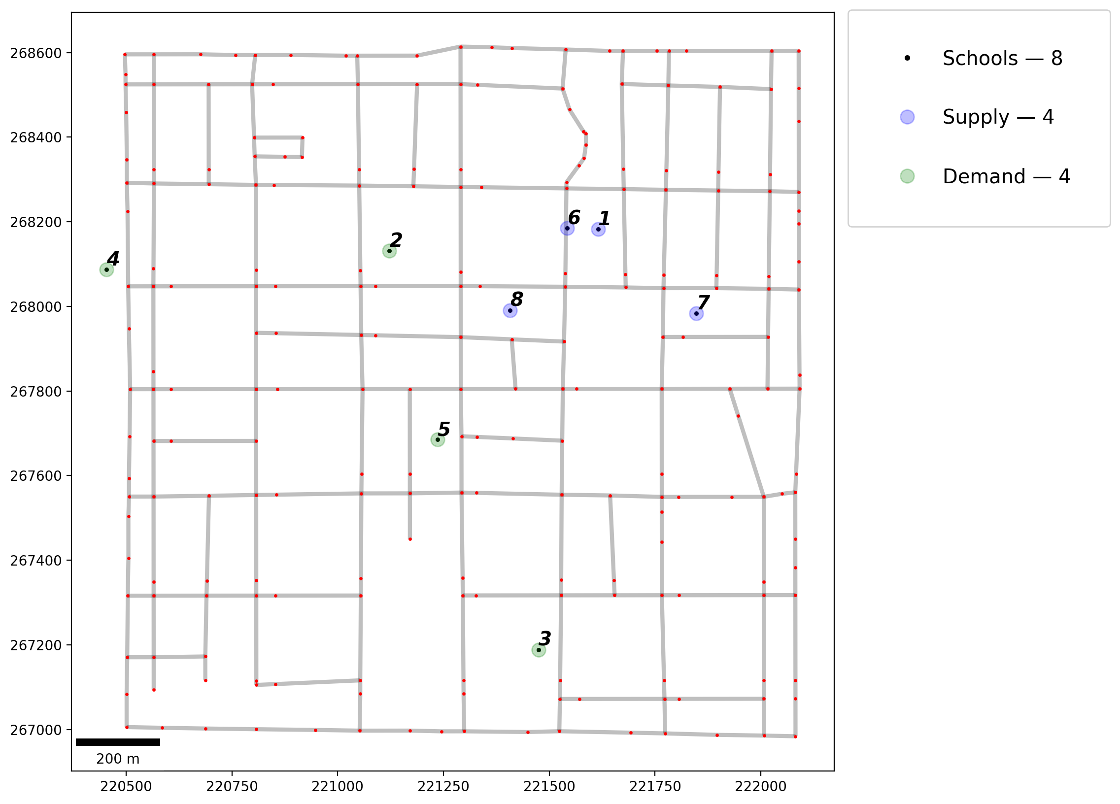
schools_supply
[14]:
| POLYID | geometry | |
|---|---|---|
| supply | ||
| 0 | 1 | POINT (221615.157 268183.063) |
| 5 | 6 | POINT (221542.706 268185.028) |
| 6 | 7 | POINT (221847.882 267983.231) |
| 7 | 8 | POINT (221406.839 267990.801) |
Schools - demand nodes
[15]:
schools_demand = schools[schools["POLYID"].isin(demand_schools)]
schools_demand.index.name = "demand"
schools_demand
[15]:
| POLYID | geometry | |
|---|---|---|
| demand | ||
| 1 | 2 | POINT (221122.271 268131.466) |
| 2 | 3 | POINT (221474.669 267188.462) |
| 3 | 4 | POINT (220453.142 268087.516) |
| 4 | 5 | POINT (221235.835 267685.028) |
Instantiate a network object
[16]:
ntw = spaghetti.Network(in_data=streets)
vertices, arcs = spaghetti.element_as_gdf(ntw, vertices=True, arcs=True)
Plot
[17]:
# plot network
base = arcs.plot(linewidth=3, alpha=0.25, color="k", zorder=0, figsize=(10, 10))
vertices.plot(ax=base, markersize=2, color="red", zorder=1)
# plot observations
schools.plot(ax=base, markersize=5, color="k", zorder=2)
schools_supply.plot(ax=base, markersize=100, alpha=0.25, color="b", zorder=2)
schools_demand.plot(ax=base, markersize=100, alpha=0.25, color="g", zorder=2)
# add labels
obs_labels(schools, base, 14, col="POLYID", c="k", weight="bold")
# add legend
elements = [schools, schools_supply, schools_demand]
legend(elements)
# add scale bar
scalebar = ScaleBar(1, units="m", location="lower left")
base.add_artist(scalebar);
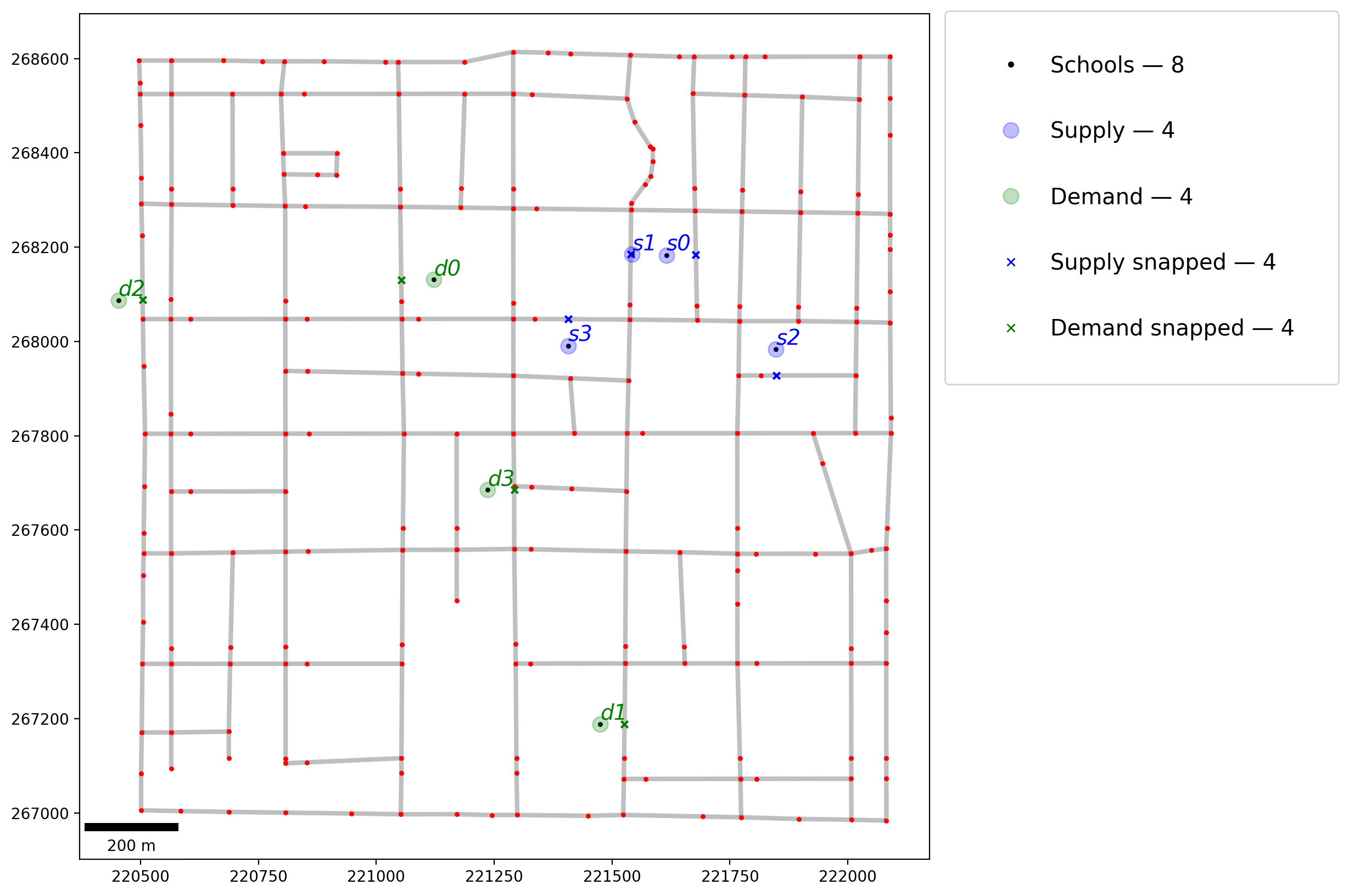
Associate both the supply and demand schools with the network and plot
[18]:
ntw.snapobservations(schools_supply, "supply")
supply = spaghetti.element_as_gdf(ntw, pp_name="supply")
supply.index.name = "supply"
supply_snapped = spaghetti.element_as_gdf(ntw, pp_name="supply", snapped=True)
supply_snapped.index.name = "supply snapped"
supply_snapped
[18]:
| id | geometry | comp_label | |
|---|---|---|---|
| supply snapped | |||
| 0 | 0 | POINT (221677.830 268184.321) | 0 |
| 1 | 1 | POINT (221539.440 268185.067) | 0 |
| 2 | 2 | POINT (221847.931 267927.691) | 0 |
| 3 | 3 | POINT (221407.196 268047.138) | 0 |
[19]:
ntw.snapobservations(schools_demand, "demand")
demand = spaghetti.element_as_gdf(ntw, pp_name="demand")
demand.index.name = "demand"
demand_snapped = spaghetti.element_as_gdf(ntw, pp_name="demand", snapped=True)
demand_snapped.index.name = "demand snapped"
demand_snapped
[19]:
| id | geometry | comp_label | |
|---|---|---|---|
| demand snapped | |||
| 0 | 0 | POINT (221053.069 268130.545) | 0 |
| 1 | 1 | POINT (221526.519 267187.875) | 0 |
| 2 | 2 | POINT (220504.720 268087.986) | 0 |
| 3 | 3 | POINT (221292.553 267685.075) | 0 |
[20]:
# plot network
base = arcs.plot(linewidth=3, alpha=0.25, color="k", zorder=0, figsize=(10, 10))
vertices.plot(ax=base, markersize=5, color="r", zorder=1)
# plot observations
schools.plot(ax=base, markersize=5, color="k", zorder=2)
supply.plot(ax=base, markersize=100, alpha=0.25, color="b", zorder=3)
supply_snapped.plot(ax=base, markersize=20, marker="x", color="b", zorder=3)
demand.plot(ax=base, markersize=100, alpha=0.25, color="g", zorder=2)
demand_snapped.plot(ax=base, markersize=20, marker="x", color="g", zorder=3)
# add labels
obs_labels(supply, base, 14, c="b")
obs_labels(demand, base, 14, c="g")
# add legend
elements += [supply_snapped, demand_snapped]
legend(elements)
# add scale bar
scalebar = ScaleBar(1, units="m", location="lower left")
base.add_artist(scalebar);
Calculate distance matrix while generating shortest path trees
[21]:
s2d, tree = ntw.allneighbordistances("supply", "demand", gen_tree=True)
s2d[:3, :3]
[21]:
array([[ 849.03401966, 1141.08317288, 1355.97131088],
       [ 705.24862712,  997.29778034, 1212.18591834],
       [ 993.39148999, 1052.63537513, 1500.3287812 ]])
[22]:
list(tree.items())[:4], list(tree.items())[-4:]
[22]:
([((0, 0), (216, 218)),
  ((0, 1), (216, 130)),
  ((0, 2), (216, 24)),
  ((0, 3), (216, 55))],
 [((3, 0), (65, 218)),
  ((3, 1), (64, 130)),
  ((3, 2), (65, 24)),
  ((3, 3), (65, 55))])
3. The Transportation Problem
Create decision variables for the supply locations and amount to be supplied
[23]:
supply["dv"] = supply["id"].apply(lambda _id: "s_%s" % _id)
supply["s_i"] = amount_supply
supply
[23]:
| id | geometry | comp_label | dv | s_i | |
|---|---|---|---|---|---|
| supply | |||||
| 0 | 0 | POINT (221615.157 268183.063) | 0 | s_0 | 20 |
| 1 | 1 | POINT (221542.706 268185.028) | 0 | s_1 | 30 |
| 2 | 2 | POINT (221847.882 267983.231) | 0 | s_2 | 15 |
| 3 | 3 | POINT (221406.839 267990.801) | 0 | s_3 | 35 |
Create decision variables for the demand locations and amount to be received
[24]:
demand["dv"] = demand["id"].apply(lambda _id: "d_%s" % _id)
demand["d_j"] = amount_demand
demand
[24]:
| id | geometry | comp_label | dv | d_j | |
|---|---|---|---|---|---|
| demand | |||||
| 0 | 0 | POINT (221122.271 268131.466) | 0 | d_0 | 5 |
| 1 | 1 | POINT (221474.669 267188.462) | 0 | d_1 | 45 |
| 2 | 2 | POINT (220453.142 268087.516) | 0 | d_2 | 10 |
| 3 | 3 | POINT (221235.835 267685.028) | 0 | d_3 | 40 |
Solve the Transportation Problem
Note: shipping costs are in meters per microscope
[25]:
s, d, s_i, d_j = supply["dv"], demand["dv"], supply["s_i"], demand["d_j"]
trans_prob = TransportationProblem(s, d, s2d, s_i, d_j)
Welcome to the CBC MILP Solver
Version: Trunk
Build Date: Oct 28 2021

Starting solution of the Linear programming problem using Primal Simplex

Minimized shipping costs: 84595.7958

Shipping decisions:
         x_0,3 20.0
         x_1,1 30.0
         x_2,1 15.0
         x_3,0 5.0
         x_3,2 10.0
         x_3,3 20.0
Linear program (compare to its formulation in the Introduction)
[26]:
trans_prob.print_lp()
 \Problem name:  TransportationProblem

Minimize
OBJROW: 849.03402 x_0,0 + 1141.08317 x_0,1 + 1355.97131 x_0,2 + 884.73265 x_0,3 + 705.24863 x_1,0 + 997.29778 x_1,1 + 1212.18592 x_1,2 + 740.94726 x_1,3 + 993.39149 x_2,0 + 1052.63538 x_2,1
 + 1500.32878 x_2,2 + 796.28486 x_2,3 + 435.89351 x_3,0 + 989.11627 x_3,1 + 942.83080 x_3,2 + 479.24516 x_3,3
Subject To
supply(0):  x_0,0 + x_0,1 + x_0,2 + x_0,3 <= 20
supply(1):  x_1,0 + x_1,1 + x_1,2 + x_1,3 <= 30
supply(2):  x_2,0 + x_2,1 + x_2,2 + x_2,3 <= 15
supply(3):  x_3,0 + x_3,1 + x_3,2 + x_3,3 <= 35
demand(0):  x_0,0 + x_1,0 + x_2,0 + x_3,0 >= 5
demand(1):  x_0,1 + x_1,1 + x_2,1 + x_3,1 >= 45
demand(2):  x_0,2 + x_1,2 + x_2,2 + x_3,2 >= 10
demand(3):  x_0,3 + x_1,3 + x_2,3 + x_3,3 >= 40
Bounds
End
Extract all network shortest paths
[27]:
paths = ntw.shortest_paths(tree, "supply", "demand")
paths_gdf = spaghetti.element_as_gdf(ntw, routes=paths)
paths_gdf.head()
[27]:
| geometry | O | D | id | |
|---|---|---|---|---|
| 0 | LINESTRING (221677.830 268184.321, 221680.004 ... | 0 | 0 | (0, 0) |
| 1 | LINESTRING (221677.830 268184.321, 221680.004 ... | 0 | 1 | (0, 1) |
| 2 | LINESTRING (221677.830 268184.321, 221680.004 ... | 0 | 2 | (0, 2) |
| 3 | LINESTRING (221677.830 268184.321, 221680.004 ... | 0 | 3 | (0, 3) |
| 4 | LINESTRING (221539.440 268185.067, 221538.155 ... | 1 | 0 | (1, 0) |
Extract the shipping paths
[28]:
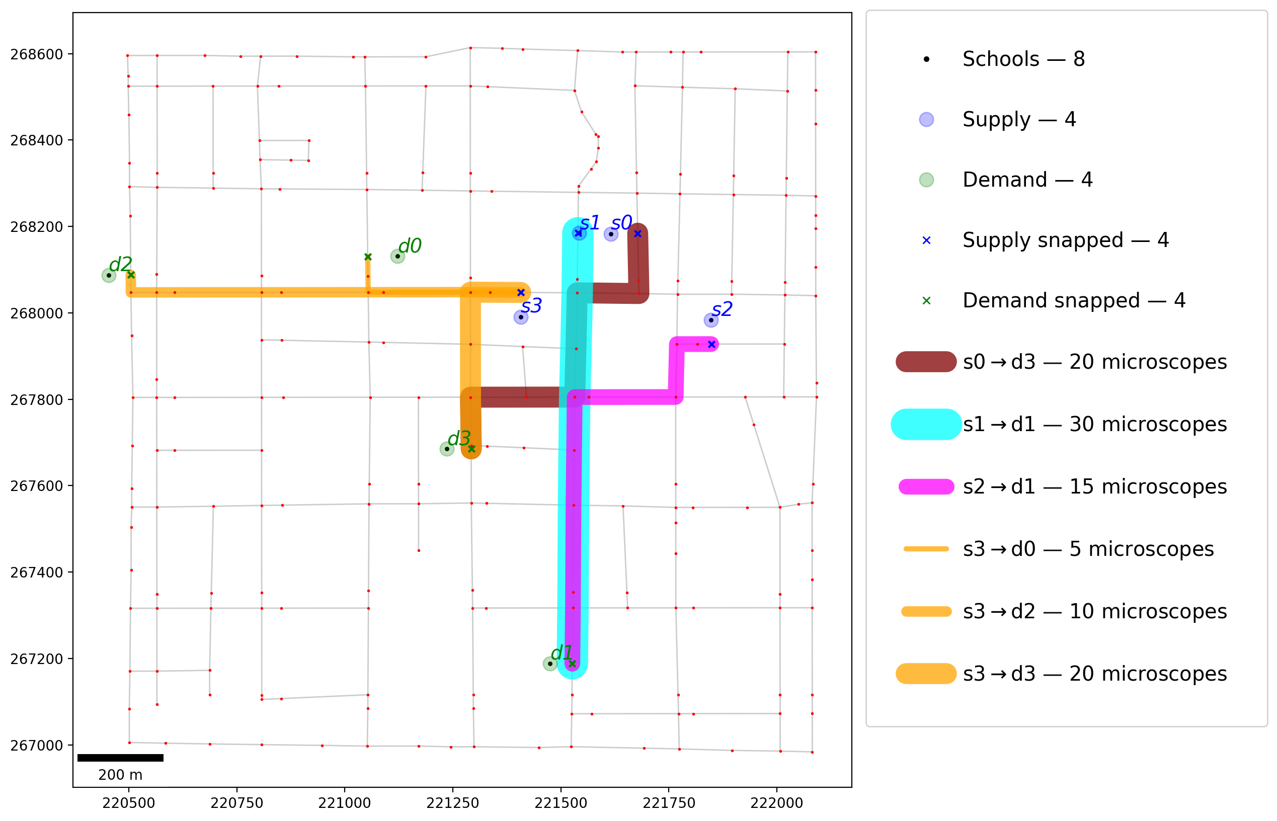
shipments = trans_prob.extract_shipments(paths_gdf, "id")
shipments
[28]:
| geometry | O | D | id | ship | |
|---|---|---|---|---|---|
| 3 | LINESTRING (221677.830 268184.321, 221680.004 ... | 0 | 3 | (0, 3) | 20 |
| 5 | LINESTRING (221539.440 268185.067, 221538.155 ... | 1 | 1 | (1, 1) | 30 |
| 9 | LINESTRING (221847.931 267927.691, 221815.862 ... | 2 | 1 | (2, 1) | 15 |
| 12 | LINESTRING (221407.196 268047.138, 221336.616 ... | 3 | 0 | (3, 0) | 5 |
| 14 | LINESTRING (221407.196 268047.138, 221336.616 ... | 3 | 2 | (3, 2) | 10 |
| 15 | LINESTRING (221407.196 268047.138, 221336.616 ... | 3 | 3 | (3, 3) | 20 |
Plot optimal shipping schedule
[29]:
# plot network
base = arcs.plot(alpha=0.2, linewidth=1, color="k", figsize=(10, 10), zorder=0)
vertices.plot(ax=base, markersize=1, color="r", zorder=2)
# plot observations
schools.plot(ax=base, markersize=5, color="k", zorder=2)
supply.plot(ax=base, markersize=100, alpha=0.25, color="b", zorder=3)
supply_snapped.plot(ax=base, markersize=20, marker="x", color="b", zorder=3)
demand.plot(ax=base, markersize=100, alpha=0.25, color="g", zorder=2)
demand_snapped.plot(ax=base, markersize=20, marker="x", color="g", zorder=3)
# plot shipments
plot_shipments(shipments.groupby("O"), base)
# add labels
obs_labels(supply, base, 14, c="b")
obs_labels(demand, base, 14, c="g")
# add legend
elements += [shipments.groupby("O")]
legend(elements)
# add scale bar
scalebar = ScaleBar(1, units="m", location="lower left")
base.add_artist(scalebar);