This page was generated from notebooks/network-spatial-dependence.ipynb.
Interactive online version:
![]()
If any part of this notebook is used in your research, please cite with the reference found in README.md.
Network-constrained spatial dependence
Demonstrating cluster detection along networks with the Global Auto K function
Author: James D. Gaboardi jgaboardi@gmail.com
This notebook is an advanced walk-through for:
Understanding the global auto K function with an elementary geometric object
Basic examples with synthetic data
Empirical examples
[1]:
%config InlineBackend.figure_format = "retina"
[2]:
%load_ext watermark
%watermark
Last updated: 2022-11-01T23:12:46.794663-04:00

Python implementation: CPython
Python version       : 3.10.6
IPython version      : 8.6.0

Compiler    : Clang 13.0.1
OS          : Darwin
Release     : 22.1.0
Machine     : x86_64
Processor   : i386
CPU cores   : 8
Architecture: 64bit
[3]:
import geopandas
import libpysal
import matplotlib
import matplotlib_scalebar
from matplotlib_scalebar.scalebar import ScaleBar
import numpy
import spaghetti

%matplotlib inline
%watermark -w
%watermark -iv
Watermark: 2.3.1

json               : 2.0.9
numpy              : 1.23.4
libpysal           : 4.6.2
matplotlib         : 3.6.1
spaghetti          : 1.6.8
geopandas          : 0.12.1
matplotlib_scalebar: 0.8.0
/Users/the-gaboardi/miniconda3/envs/py310_spgh_dev/lib/python3.10/site-packages/spaghetti/network.py:39: FutureWarning: The next major release of pysal/spaghetti (2.0.0) will drop support for all ``libpysal.cg`` geometries. This change is a first step in refactoring ``spaghetti`` that is expected to result in dramatically reduced runtimes for network instantiation and operations. Users currently requiring network and point pattern input as ``libpysal.cg`` geometries should prepare for this simply by converting to ``shapely`` geometries.
  warnings.warn(f"{dep_msg}", FutureWarning)
The K function considers all pairwise distances of nearest neighbors to determine the existence of clustering, or lack thereof, over a delineated range of distances. For further description see O’Sullivan and Unwin (2010) and Okabe and Sugihara (2012).
D. O’Sullivan and D. J. Unwin. Point Pattern Analysis, chapter 5, pages 121–156. John Wiley & Sons, Ltd, 2010. doi:10.1002/9780470549094.ch5.
Atsuyki Okabe and Kokichi Sugihara. Network K Function Methods, chapter 6, pages 119–136. John Wiley & Sons, Ltd, 2012. doi:10.1002/9781119967101.ch6.
1. A demonstration of clustering
Results plotting helper function
[4]:
def plot_k(k, _arcs, df1, df2, obs, scale=True, wr=[1, 1.2], size=(14, 7)):
    """Plot a Global Auto K-function and spatial context."""
    def function_plot(f, ax):
        """Plot a Global Auto K-function."""
        ax.plot(k.xaxis, k.observed, "b-", linewidth=1.5, label="Observed")
        ax.plot(k.xaxis, k.upperenvelope, "r--", label="Upper")
        ax.plot(k.xaxis, k.lowerenvelope, "k--", label="Lower")
        ax.legend(loc="best", fontsize="x-large")
        title_text = "Global Auto $K$ Function: %s\n" % obs
        title_text += "%s steps, %s permutations," % (k.nsteps, k.permutations)
        title_text += " %s distribution" % k.distribution
        f.suptitle(title_text, fontsize=25, y=1.1)
        ax.set_xlabel("Distance $(r)$", fontsize="x-large")
        ax.set_ylabel("$K(r)$", fontsize="x-large")

    def spatial_plot(ax):
        """Plot spatial context."""
        base = _arcs.plot(ax=ax, color="k", alpha=0.25)
        df1.plot(ax=base, color="g", markersize=30, alpha=0.25)
        df2.plot(ax=base, color="g", marker="x", markersize=100, alpha=0.5)
        carto_elements(base, scale)

    sub_args = {"gridspec_kw":{"width_ratios": wr}, "figsize":size}
    fig, arr = matplotlib.pyplot.subplots(1, 2, **sub_args)
    function_plot(fig, arr[0])
    spatial_plot(arr[1])
    fig.tight_layout()

def carto_elements(b, scale):
    """Add/adjust cartographic elements."""
    if scale:
        kw = {"units":"ft", "dimension":"imperial-length", "fixed_value":1000}
        b.add_artist(ScaleBar(1, **kw))
    b.set(xticklabels=[], xticks=[], yticklabels=[], yticks=[]);
Equilateral triangle
[5]:
def equilateral_triangle(x1, y1, x2, mids=True):
    """Return an equilateral triangle and its side midpoints."""
    x3 = (x1+x2)/2.
    y3 = numpy.sqrt((x1-x2)**2 - (x3-x1)**2) + y1
    p1, p2, p3 = (x1, y1), (x2, y1), (x3, y3)
    eqitri = libpysal.cg.Chain([p1, p2, p3, p1])
    if mids:
        eqvs = eqitri.vertices[:-1]
        eqimps, vcount = [], len(eqvs),
        for i in range(vcount):
            for j in range(i+1, vcount):
                (_x1, _y1), (_x2, _y2) = eqvs[i], eqvs[j]
                mp = libpysal.cg.Point(((_x1+_x2)/2., (_y1+_y2)/2.))
                eqimps.append(mp)
    return eqitri, eqimps
[6]:
eqtri_sides, eqtri_midps = equilateral_triangle(0., 0., 6., 1)
ntw = spaghetti.Network(eqtri_sides)
ntw.snapobservations(eqtri_midps, "eqtri_midps")
[7]:
vertices_df, arcs_df = spaghetti.element_as_gdf(
    ntw, vertices=ntw.vertex_coords, arcs=ntw.arcs
)
eqv = spaghetti.element_as_gdf(ntw, pp_name="eqtri_midps")
eqv_snapped = spaghetti.element_as_gdf(ntw, pp_name="eqtri_midps", snapped=True)
eqv_snapped
[7]:
| id | geometry | comp_label | |
|---|---|---|---|
| 0 | 0 | POINT (3.00000 0.00000) | 0 |
| 1 | 1 | POINT (1.50000 2.59808) | 0 |
| 2 | 2 | POINT (4.50000 2.59808) | 0 |
[8]:
numpy.random.seed(0)
kres = ntw.GlobalAutoK(
    ntw.pointpatterns["eqtri_midps"],
    nsteps=100,
    permutations=100)
plot_k(kres, arcs_df, eqv, eqv_snapped, "eqtri_mps", wr=[1, 1.8], scale=False)
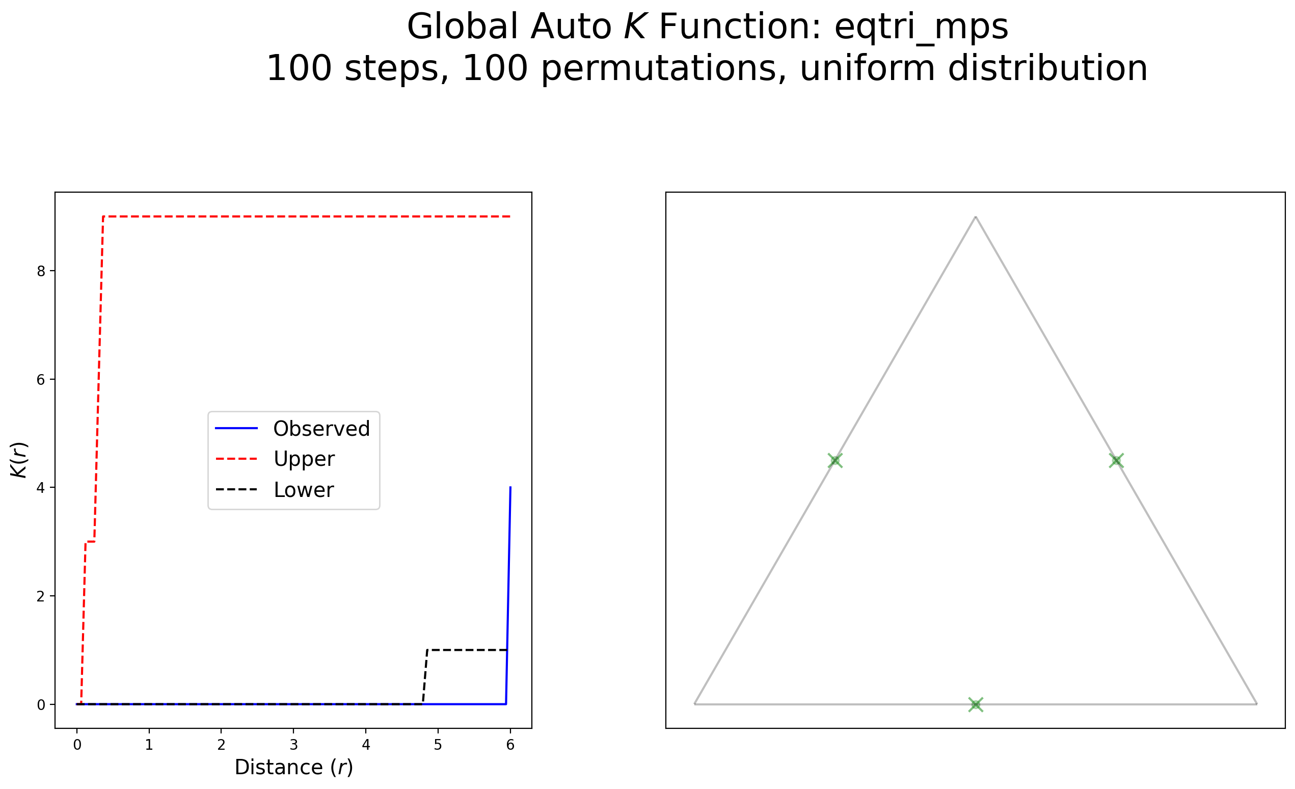
Interpretation:
This example demonstrates a complete lack of clustering with a strong indication of dispersion when approaching 5 units of distance.
2. Synthetic examples
Regular lattice — distinguishing visual clustering from statistical clustering
[9]:
bounds = (0,0,3,3)
h, v = 2, 2
lattice = spaghetti.regular_lattice(bounds, h, nv=v, exterior=True)
ntw = spaghetti.Network(in_data=lattice)
Network arc midpoints: statistical clustering
[10]:
midpoints = []
for chain in lattice:
    (v1x, v1y), (v2x, v2y) = chain.vertices
    mp = libpysal.cg.Point(((v1x+v2x)/2., (v1y+v2y)/2.))
    midpoints.append(mp)
ntw.snapobservations(midpoints, "midpoints")
All observations on two network arcs: visual clustering
[11]:
npts = len(midpoints) * 2
xs = [0.0] * npts + [2.0] * npts
ys = list(numpy.linspace(0.4,0.6, npts)) + list(numpy.linspace(2.1,2.9, npts))
pclusters = [libpysal.cg.Point(xy) for xy in zip(xs,ys)]
ntw.snapobservations(pclusters, "pclusters")
[12]:
vertices_df, arcs_df = spaghetti.element_as_gdf(ntw, vertices=True, arcs=True)
midpoints = spaghetti.element_as_gdf(ntw, pp_name="midpoints", snapped=True)
pclusters = spaghetti.element_as_gdf(ntw, pp_name="pclusters", snapped=True)
Visual clustering
[13]:
numpy.random.seed(0)
kres = ntw.GlobalAutoK(ntw.pointpatterns["pclusters"], nsteps=100, permutations=100)
plot_k(kres, arcs_df, pclusters, pclusters, "pclusters", wr=[1, 1.8], scale=False)
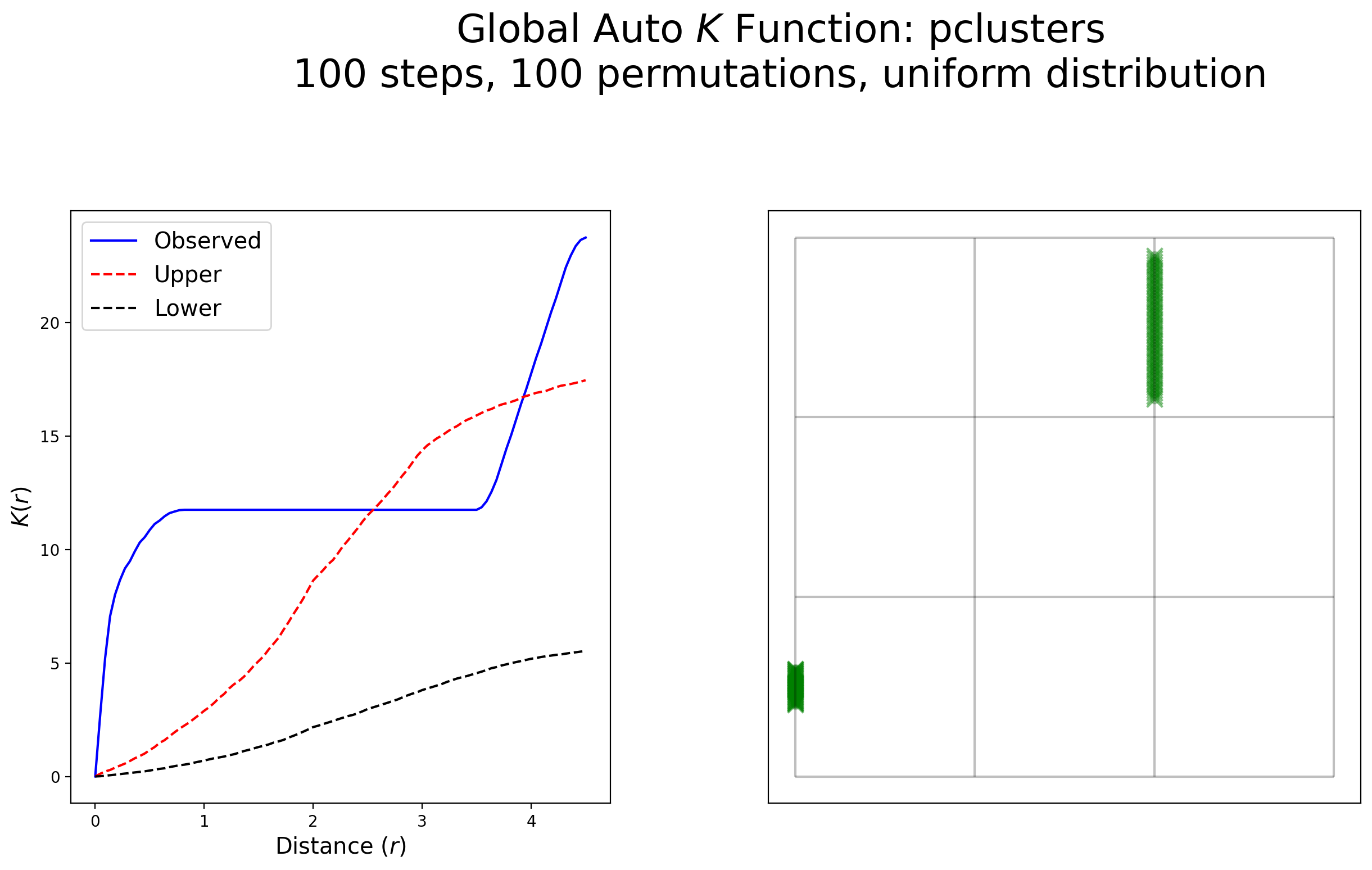
Interpretation:
This example exhibits a high degree of clustering within 1 unit of distance followed by a complete lack of clustering, then a strong indication of clustering around 3.5 units of distance and above. Both colloquilly and statistically, this pattern is clustered.
Statistical clustering
[14]:
numpy.random.seed(0)
kres = ntw.GlobalAutoK(ntw.pointpatterns["midpoints"], nsteps=100, permutations=100)
plot_k(kres, arcs_df, midpoints, midpoints, "midpoints", wr=[1, 1.8], scale=False)
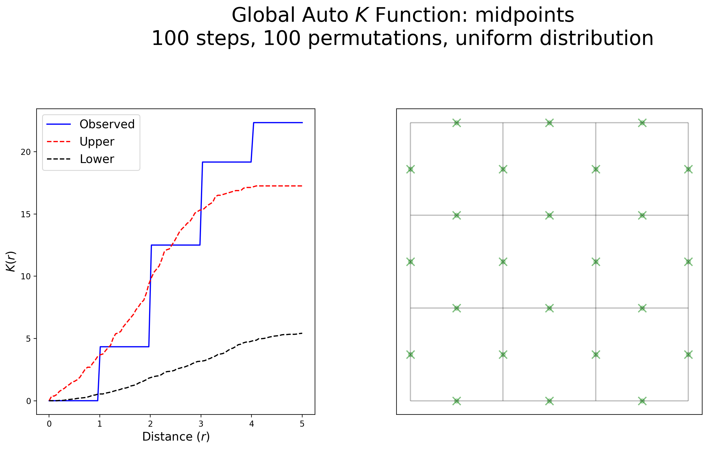
Interpretation:
This example exhibits no clustering within 1 unit of distance followed by large increases in clustering at each 1-unit increment. After 3 units of distance, this pattern is highly clustered. Statistically speaking, this pattern is clustered, but not colloquilly.
3. Empircal examples
Instantiate the network from a .shp file
[15]:
ntw = spaghetti.Network(in_data=libpysal.examples.get_path("streets.shp"))
vertices_df, arcs_df = spaghetti.element_as_gdf(
    ntw, vertices=ntw.vertex_coords, arcs=ntw.arcs
)
Associate the network with point patterns
[16]:
for pp_name in ["crimes", "schools"]:
    pp_shp = libpysal.examples.get_path("%s.shp" % pp_name)
    ntw.snapobservations(pp_shp, pp_name, attribute=True)
ntw.pointpatterns
[16]:
{'crimes': <spaghetti.network.PointPattern at 0x165388c10>,
 'schools': <spaghetti.network.PointPattern at 0x16564f670>}
Empircal — schools
[17]:
schools = spaghetti.element_as_gdf(ntw, pp_name="schools")
schools_snapped = spaghetti.element_as_gdf(ntw, pp_name="schools", snapped=True)
[18]:
numpy.random.seed(0)
kres = ntw.GlobalAutoK(
    ntw.pointpatterns["schools"],
    nsteps=100,
    permutations=100)
plot_k(kres, arcs_df, schools, schools_snapped, "schools")
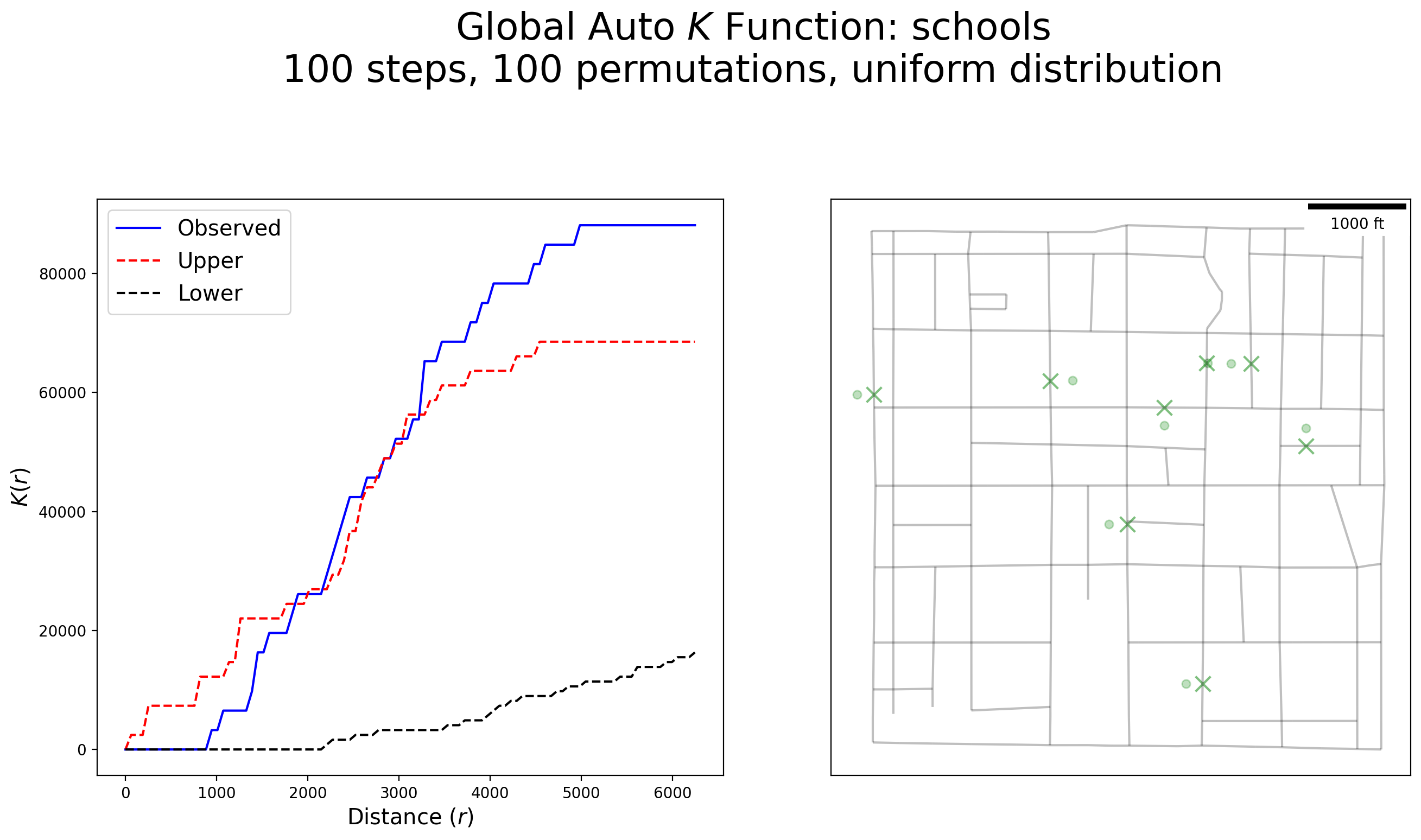
Interpretation:
Schools exhibit no clustering until roughly 1,000 feet then display more clustering up to approximately 3,000 feet, followed by high clustering up to 6,000 feet.
Empircal — crimes
[19]:
crimes = spaghetti.element_as_gdf(ntw, pp_name="crimes")
crimes_snapped = spaghetti.element_as_gdf(ntw, pp_name="crimes", snapped=True)
[20]:
numpy.random.seed(0)
kres = ntw.GlobalAutoK(
    ntw.pointpatterns["crimes"],
    nsteps=100,
    permutations=100)
plot_k(kres, arcs_df, crimes, crimes_snapped, "crimes")
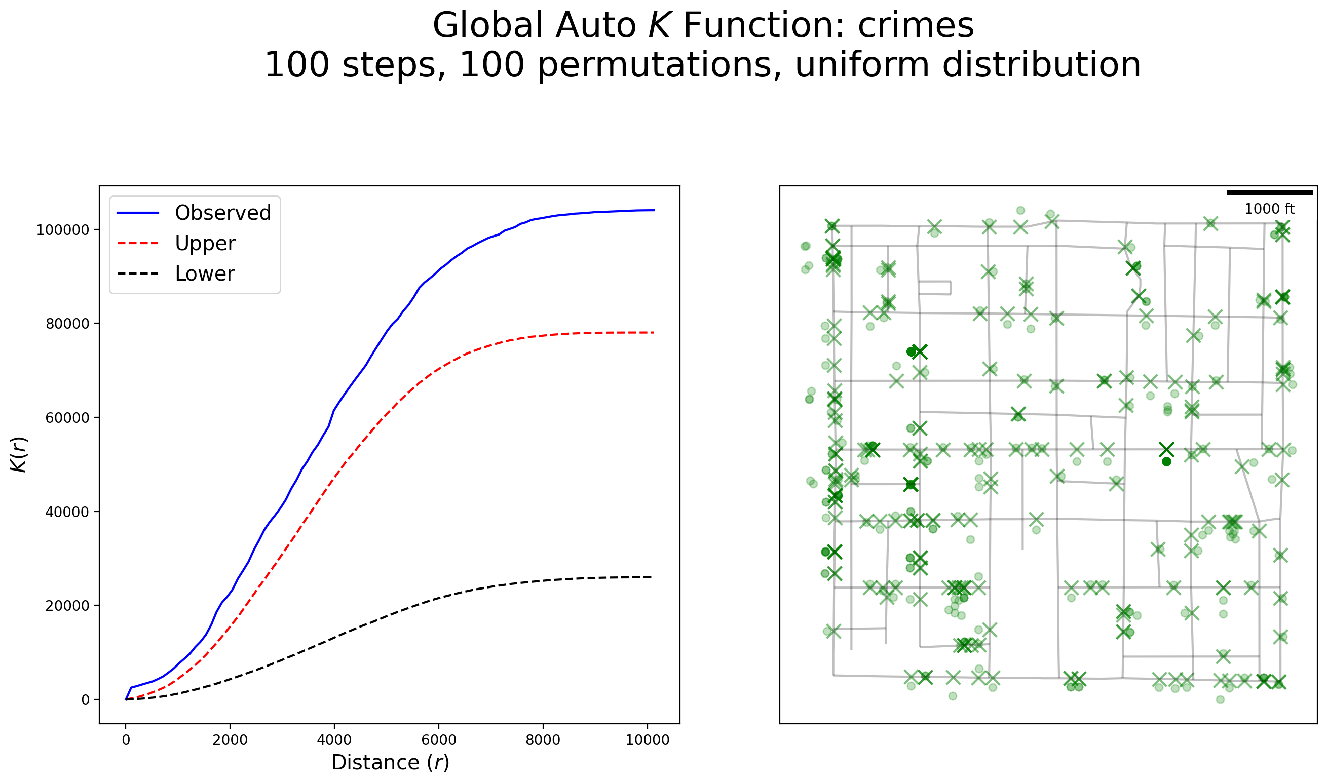
Interpretation:
There is strong evidence to suggest crimes are clustered at all distances along the network, but more so within several feet of each other and at 10,000 feet.