Working with Raster data
Geographic data comes in two common representations.
The first, called vector data, refers to a representation where coordinates are indexed in continuous space with a position vector. Coordinates have no dimension, but are combined togehter to form geometries, such as points, lines, and polygons. These combinations have certain rules for how they can be combined into geometries.
In the previous notebook, we worked mainly with vector geometries, although the basemaps we used to construct better maps were raster representations of geographical data. Raster representations of geographic data are like images; they are composed of small identical polygons (usually squares) with a single value. Usually, Raster datasets map naturally to an array, where each element is the observed value at a given cell. If there are multiple sensed values at each site, then each value is assigned a band. In geography, this terminology comes from early work in digital aerial photography applications, where each band represented an electromagnetic wavelength (such as infrared, red, green, blue, ultraviolet, etc.) recorded by an aerial sensor. This is opposed to vector data, which grew out of applications in computer graphics.
Below, we discuss a few methods for working with rasters, as well as ways to combine rasters.
Reading & Writing raster data using Rasterio
There is a wide variety of raster data processing methods in Python, given the extensive ecosystem of satellite imagery and analysis tools for Python. For large raster datasets, the pangeo project may be of interest. However, many common processing pipelines rely on rasterio, which is built on the GEOS library, like PostGIS and shapely, which underlies geopandas.
import rasterio # the GEOS-based raster package
import numpy # the array computation library
import geopandas # the GEOS-based vector package
import contextily # the package for fetching basemaps
import matplotlib.pyplot as plt # the visualization package
%matplotlib inline
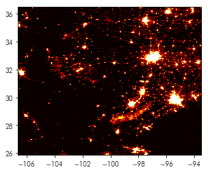
To get started with rasterio, you should use rasterio.open() to create a “dataset” (or, sometimes called a “file handle”). Below, we’ll open a dataset containing the nighttime lights sensed from Texas:
nightlight_file = rasterio.open('../data/txlights.tif')
The rasterio.open() command works similarly to the built-in Python open command, but offers different methods that are relevant to raster data. For instance, the read() method takes an argument for the band which you want to read from the data (indexed from 1):
nightlights = nightlight_file.read(1)
as well as quite a few other attributes, such as:
nightlight_file.crs # the coordinate reference system
nightlight_file.shape # the shape of the raster image
When a band is read(), the values from the band are stored in memory as a numpy.ndarray. This means that the band read in from txnightlights.tiff can be operated on like a typical numpy array. To show the data, we can use the same approach as when we were using contextily tiles:
plt.imshow(nightlights, cmap='hot')

For multi-band images, the rasterio.plot.show() method can also provide detailed, multi-band plots:
from rasterio import plot as rioplot
rioplot.show(nightlight_file, cmap='hot')
Looking carefully, you’ll note that the rasterio.plot.show() function also sets the axis correctly to latitude (for the yaxis) and longitude (for the xaxis). To do this correctly for the raster dataset, we would need to construct its extent. This is already provided in one form by nightlight_file:
nightlight_file.bounds
But, matplotlib and geographic packages like rasterio and geopandas use different ordering conventions for their bounding box information.
geographic information systems (bounds): (west, south, north, east) matplotlib (extent): (west, east, south, north)
We will consistently use the term bounds or bound form to refer to the top ordering, and extent or extent form when referring to the bottom ordering. As such, we must re-arrange the nightlight_file.bounds to extent form, expected by matplotlib:
nightlight_extent = numpy.asarray(nightlight_file.bounds)[[0,2,1,3]]
Then, we can use it in imshow to correct the axis labels:
plt.imshow(nightlights, cmap='hot', extent=nightlight_extent)

Subsetting Rasters
Often, rasters and vectors have to be used together. It’s often the case that many kinds of geographical processes are being analyzed in a single area of study, so more than one kind of representation is needed for a given analytical purpose. Below, we’ll show a few ways to use vector features (such as polygons or points) together with a raster, such as the nightlight data shown above.
For instance, our data shows the nightlights for all of Texas. However, our other data sources used in the previous notebooks in this workshop focus explicitly on the city of Austin. To focus the raster down to Austin, we can use the neighborhoods data, which we converted into geographic information earlier.
neighborhoods = geopandas.read_file('../data/neighborhoods.gpkg')
The neighborhoods data, like any data stored in a geopandas.GeoDataFrame, has its total_bounds recomputed on the fly. Thus, the bounding box for our neighborhoods in Austin (which is a good proxy for the bounding box of Austin itself) is the total_bounds of our neighborhood dataframe:
austin_bbox = neighborhoods.total_bounds
Subsetting raster data in rasterio is easiest to do before it is read into memory (although it is possible to do so after read()). Subsetting data requires a rasterio.windows.Window object to be built that describes the area to focus on. There are many helper functions to build windows, but the simplest is:
nightlight_file.window?
This takes the coordinates from a bounding box and provides a rasterio.windows.Window object. We can use it directly from our austin_bbox data using *, the unpack operator in Python:
austin_window = nightlight_file.window(*austin_bbox)
Now, when we read() in our data, we can use this rasterio.windows.Window object to only read the data we want to analyze: that within the bounds of the neighborhoods in Austin:
austin_nightlights = nightlight_file.read(1, window=austin_window)
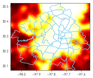
To see what this looks like together, we can make a plot that contains both raster and vector data in the same fashion we have done with basemaps in contextily:
plt.imshow(austin_nightlights, extent=austin_bbox[[0,2,1,3]], cmap='hot')
neighborhoods.boundary.plot(ax=plt.gca(), color='skyblue')
Writing out raster geodata is somewhat more complex. Since the actual raster contains much less information about the geographic structure of the raster than, say, a geopandas.GeoDataFrame, it is necessary to supply quite a bit more information to the rasterio.open() and rasterio.write() functions. In most cases, it is necessary to supply:
- the size of the image in pixels (since the image may differ from the size of the array being used to write to the image)
- the coordinate reference system for the image (since the
numpy.ndarrayhas no information about coordinate reference systems inside of it) - the “transformation”, which is the
rasterio.Affineclass that describes the affine transform matrix of the array that is required to “fit” into the coordinate reference system provided.
Again, fotunately, there are helper functions in rasterio to construct these things. For instance, as we saw above, the coordinate reference system for an image is stored in:
nightlight_file.crs
And, in many cases, the transform can be constructed directly from a rasterio.window.Window object (assuming that this is truly the transform of the raster).
austin_transform = nightlight_file.window_transform(austin_window)
Thus, to write our new raster out that focues exlusively on Austin, we can use the following open() & write() calls:
with rasterio.open('../data/austinlights.tif', #filename
                   'w', # file mode, with 'w' standing for "write"
                   driver='GTiff', # format to write the data
                   height=austin_nightlights.shape[0], # height of the image, often the height of the array
                   width=austin_nightlights.shape[1], # width of the image, often the width of the array
                   count=1, # the number of bands to write
                   dtype=rasterio.ubyte, # the dtype of the data, usually `ubyte` if data is stored in integers
                   crs=nightlight_file.crs, # the coordinate reference system of the data
                   transform=austin_transform # the affine transformation for the image
                  ) as outfile:
    outfile.write(austin_nightlights, indexes=1) # write the `austin_nightlights` as the first band
Working between representations
Often, it’s necessary to move data between representations. A few common operations are required to work fluently between representations:
- polygonizing rasters: drawing vector polygons around cell patches that have a given value
- rasterizing vector features: converting vector values into a raster, at a given, prespecified resolution.
- zonal statistics: computing statistics about raster cells that intersect vector features. When done with point-based vector features, this is often called sampling or resampling from the raster.
converting between vector and raster representations is often fairly straightforward, since these involve very well-specified transformations of the input data. Zonal statistics, however, are very often required in analytical applications, and can occasionally be complex or confusing to construct. As such, we’ll cover techniques for computing zonal statistics about polygon and point features in an efficient fashion.
Zonal Statistics
For simple, direct applications, there is a dedicated package in python (called python-rasterstats) for doing zonal statistics on raster data:
import rasterstats
For computing raster statistics from numpy arrays in memory, it is necessary to specify the affine transform (using the affine argument) that relates the array to the geometry:
rasterstats.zonal_stats(neighborhoods.geometry.head(), austin_nightlights,
                        affine=austin_transform)
To compute your own user-defined functions, you can pass them along as well inside of the add_stats argument. Further, the stats keyword argument can also specify which statistics you are interested in computing, stated in a string. Supported options are detailed here, but include (at the time of writing):
- min
- max
- mean
- count
- sum
- std
- median
- majority (aka most common value, in the case where no majority exists)
- minority (aka least common value)
- unique
- range
- nodata
- percentile
Ones stated in italics are computed by default, as you see in the first computation. So, for instance, to do a special computation on the input, we might use something like:
from scipy.stats import skew

def flatskew(x):
    """
    Compute the skewness of all values in an input masked array
    """
    return skew(x.data, axis=None)
rasterstats.zonal_stats(neighborhoods.geometry.head(), austin_nightlights,
                        affine=austin_transform, stats=' ',
                        add_stats=dict(skew=flatskew))
Notably, as we’ll discuss in detail below when we get into how zonal stats work, the functions passed through add_stats must accept masked arrays as input.
The rasterstats package is flexible, but it is often better to work directly with rasterio. The interpolation strategies used in rasterstats for converting raster features to vector values can yield unexpected results. Using rasterio directly, you can ensure that your results are exactly what you intend.
Therefore, we’ll walk through a little bit of how you might implement zonal statistics by yourself using rasterio.mask.
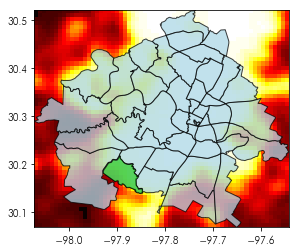
A mask is like a filter on the values of an array. Using a mask, you can select only pixels that intersect a given shape. So, for example, consider the first neighborhood in our neighborhoods data (shown in green):
ax = neighborhoods.geometry.plot(color='lightblue', alpha=.75, edgecolor='k')
neighborhoods.geometry[[0]].plot(color='limegreen', ax=ax, alpha=.75, edgecolor='k')
ax.imshow(austin_nightlights, extent=austin_bbox[[0,2,1,3]], cmap='hot')
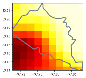
Using the mask module, we can focus the raster onto cells that are around that feature. So, for instance, in the zoomed-in plot of that neighborhood below:
test_shape = neighborhoods.geometry[[0]]
plt.imshow(austin_nightlights, extent=neighborhoods.total_bounds[[0,2,1,3]], cmap='hot')
test_shape.boundary.plot(ax = plt.gca(), color='slategrey', linewidth=3)
plt.axis(test_shape.total_bounds[[0,2,1,3]])
The rasterio.mask function helps us to select only the cells that intersect the geometry itself.
from rasterio.mask import mask
rasterio masks operate on the filehandle, rather than on an array. This improves efficiency, because the whole raster does not have to be read into memory. In the simplest case, using the mask function on a single geomery works as follows:
masked, mask_transform = mask(dataset=nightlight_file,
                              shapes=test_shape, crop=True)
The crop() argument ensures that the outputted raster only covers the extent of the input features. When crop() is false (which occurs by default), the whole raster shape is retained. We use it here to avoid reading in the whole raster, and to make it easier to visualize the cropped component.
The mask function returns an array with the shape (n_bands, n_rows, n_columns). Thus, when working with a single band, the mask function will output an array that has an “extra” dimension; the array will be three-dimensional despite the output only having two effective dimensions. So, we must use squeeze() to remove extra dimensions that only have one element:
print('initial shape: {}'.format(masked.shape)) # we only need the (10,11) array
masked = masked.squeeze()
print('final shape: {}'.format(masked.shape))
Then, to visualize how this masking works, we can plot the masked array and the polygon used to build the mask together:
plt.imshow(masked.squeeze(), cmap='hot', extent=test_shape.total_bounds[[0,2,1,3]])
test_shape.boundary.plot(ax=plt.gca(), color='grey', linewidth=4)
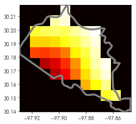
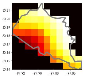
Note that this is underfilled, in that some pixels intersect the boundary of our test shape, but are not retained by the mask. Therefore, we can ensure that all intersecting pixels are retained using the all_touches argument, which will overfill the boundary and pick all cells that intersect the vector feature:
masked, mask_transform = mask(dataset=nightlight_file,
                              shapes=test_shape, crop=True, all_touched=True)
We can visualize this again in the same fashion:
plt.imshow(masked.squeeze(), cmap='hot',
           extent=test_shape.total_bounds[[0,2,1,3]])
test_shape.boundary.plot(ax=plt.gca(), color='grey', linewidth=4)
The resulting mask is a standard numpy array. To see how these look:
masked
By default, areas outside of the shape are filled with zeros. This is unfortunate for raster statistics, since a no-data value of zero will usually skew the zonal statistics. Including the zeros, the mean of this area is:
masked.mean()
However, for only the cells that are included in the selection, the mean is quite different:
masked[masked.nonzero()].mean()
To ensure that the mask does not bias towards the fill value, we can use the filled argument. When False, the array will be masked, rather than filled with a default value. This mask makes the return a numpy MaskedArray, which behaves slightly differently from a standard numpy array.
masked, mask_transform = mask(dataset=nightlight_file,
                              shapes=test_shape, crop=True,
                              all_touched=True,
                              filled=False)
plt.imshow(masked.squeeze(), cmap='hot',
           extent=test_shape.total_bounds[[0,2,1,3]])
test_shape.boundary.plot(ax=plt.gca(), color='grey', linewidth=4)
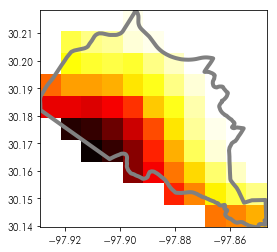
Seeing the values again, we can see that the masked array itself represents the values in a substantially different manner than the default array filled with zeros outside of the polygon:
masked
By default, methods like mean(), min(), or max() of masked arrays will return the correct result:
masked.mean()
But, more complicated statistics may need to be used directly from the numpy.ma module, rather than those used in numpy alone:
numpy.ma.median(masked)
numpy.median(masked)
Since this works for each geometry, it is possible to apply this mask function over the geometries of a GeoDataFrame and include it in a typical pandas apply chain:
def clean_mask(geom, dataset=nightlight_file, **mask_kw):
    mask_kw.setdefault('crop', True)
    mask_kw.setdefault('all_touched', True)
    mask_kw.setdefault('filled', False)
    masked, mask_transform = mask(dataset=dataset, shapes=(geom,),
                                  **mask_kw)
    return masked
neighborhoods['nightlights'] = neighborhoods.geometry.apply(clean_mask).apply(numpy.ma.median)
Now, this nightlights column contains the median nighttime light sensed within each neighborhood of Austin:
neighborhoods.nightlights.head()
To map this, we’ll first grab a basemap:
basemap, basemap_extent = contextily.bounds2img(*neighborhoods.to_crs(epsg=3857).total_bounds,
                                                zoom=10)
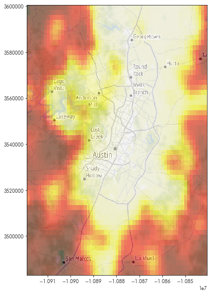
And then construct a typical map on top:
plt.figure(figsize=(10,10))
plt.imshow(basemap, extent=basemap_extent)
neighborhoods.to_crs(epsg=3857).plot('nightlights',
                                     cmap='hot', ax = plt.gca(), alpha=.75)
plt.axis(neighborhoods.to_crs(epsg=3857).total_bounds[[0,2,1,3]])
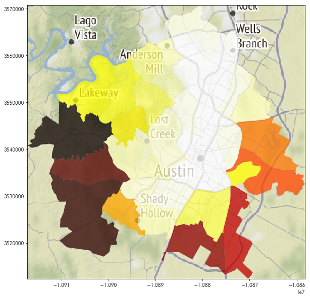
which broadly comports with our perception of what the neighborhood brightness ought look like:
plt.figure(figsize=(10,10))
plt.imshow(basemap, extent=basemap_extent)
plt.imshow(austin_nightlights, extent=basemap_extent, cmap='hot', alpha=.5)
Getting values at cells?
To get the values of a raster at specific vector points, there are a few ways this can be done. Conceptually, one could use very small buffers and apply the same zonal statistics method used above. But, this is very computationally wasteful, and it is often unclear as to how small a buffer has to be to avoid hitting a boundary between cells in the raster. Therefore, there are often dedicated functions to compute the raster value at vector coordinates.
To show this, let’s first read in the listings data we used in the previous notebook:
listings = geopandas.read_file('../data/listings.gpkg')
While the rasterstats.point_query function is available, using the .sample() method from rasterio is recommended.
To work with the rasterio.sample method, we unfortunately cannot use GeoDataFrame.geometry directly. Instead, one can use the GeoDataFrame.geometry.x and GeoDataFrame.geometry.y methods to access the x and y coordinates separately:
coordinates = numpy.vstack((listings.geometry.x.values, listings.geometry.y.values)).T
brightnesses = nightlight_file.sample(coordinates)
listings['brightness_rasterio'] = numpy.vstack(brightnesses)
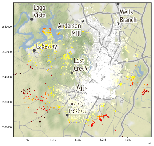
Then, we can map these values just like before:
plt.figure(figsize=(10,10))
plt.imshow(basemap, extent=basemap_extent)
listings.to_crs(epsg=3857).plot('brightness_rasterio', ax=plt.gca(),
                                marker='.', cmap='hot')
plt.axis(listings.to_crs(epsg=3857).total_bounds[[0,2,1,3]])
From here, you should now be equipped to tackle the rasters-problemset.ipynb!