%matplotlib inline

import pandas as pd
import geopandas as gpd
import libpysal as lp
import esda
import numpy as np
import matplotlib.pyplot as plt
Case Study: Gini in a bottle: Income Inequality and the Trump Vote
Read in the table and show the first three rows
pres = gpd.read_file("zip://../data/uspres.zip")
pres.head(3)
Set the Coordinate Reference System and reproject it into a suitable projection for mapping the contiguous US
hint: the epsg code useful here is 5070, for Albers equal area conic focused on North America
pres.crs = {'init':'epsg:4326'}
pres = pres.to_crs(epsg=5070)
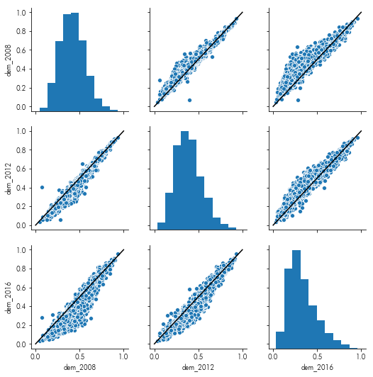
Plot each year’s vote against each other year’s vote
In this instance, it also helps to include the line ($y=x$) on each plot, so that it is clearer the directions the aggregate votes moved.
import seaborn as sns
facets = sns.pairplot(data=pres.filter(like='dem_'))
facets.map_offdiag(lambda *arg, **kw: plt.plot((0,1),(0,1), color='k'))
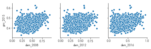
Show the relationship between the dem two-party vote and the Gini coefficient by county.
import seaborn as sns
facets = sns.pairplot(x_vars=pres.filter(like='dem_').columns,
                      y_vars=['gini_2015'], data=pres)
Compute change in vote between each subsequent election
pres['swing_2012'] = pres.eval("dem_2012 - dem_2008")
pres['swing_2016'] = pres.eval("dem_2016 - dem_2012")
pres['swing_full'] = pres.eval("dem_2016 - dem_2008")
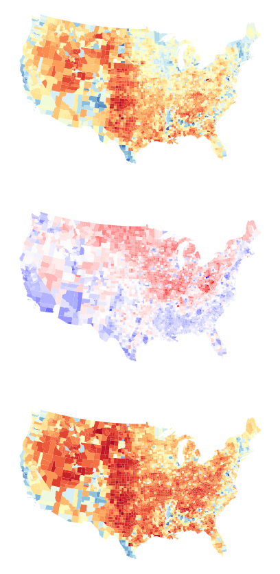
Negative swing means the Democrat voteshare in 2016 (what Clinton won) is lower than Democrat voteshare in 2008 (what Obama won). So, counties where swing is negative mean that Obama “outperformed” Clinton. Equivalently, these would be counties where McCain (in 2008) “beat” Trump’s electoral performance in 2016.
Positive swing in a county means that Clinton (in 2016) outperformed Obama (in 2008), or where Trump (in 2016) did better than McCain (in 2008).
The national average swing was around -9% from 2008 to 2016. Further, swing does not directly record who “won” the county, only which direction the county “moved.”
map the change in vote from 2008 to 2016 alongside the votes in 2008 and 2016:
f,ax = plt.subplots(3,1,
                    subplot_kw=dict(aspect='equal',
                                    frameon=False),
                    figsize=(60,15))
pres.plot('dem_2008', ax=ax[0], cmap='RdYlBu')
pres.plot('swing_full', ax=ax[1], cmap='bwr_r')
pres.plot('dem_2016', ax=ax[2], cmap='RdYlBu')
for i,ax_ in enumerate(ax):
    ax_.set_xticks([])
    ax_.set_yticks([])
Build a spatial weights object to model the spatial relationships between US counties
import libpysal as lp
w = lp.weights.Rook.from_dataframe(pres)
Note that this is just one of many valid solutions. But, all the remaining exercises are predicated on using this weight. If you choose a different weight structure, your results may differ.
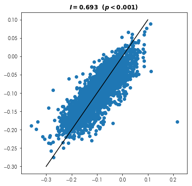
Is swing “contagious?” Do nearby counties tend to swing together?
from pysal.explore import esda as esda
np.random.seed(1)
moran = esda.moran.Moran(pres.swing_full, w)
print(moran.I)
Visually show the relationship between places’ swing and their surrounding swing, like in a scatterplot.
f = plt.figure(figsize=(6,6))
plt.scatter(pres.swing_full, lp.weights.lag_spatial(w, pres.swing_full))
plt.plot((-.3,.1),(-.3,.1), color='k')
plt.title('$I = {:.3f} \ \ (p < {:.3f})$'.format(moran.I,moran.p_sim))
Are there any outliers or clusters in swing using a Local Moran’s $I$?
np.random.seed(11)
lmos = esda.moran.Moran_Local(pres.swing_full, w,
                              permutations=70000) #min for a bonf. bound
(lmos.p_sim <= (.05/len(pres))).sum()
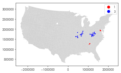
Where are these outliers or clusters?
f = plt.figure(figsize=(10,4))
ax = plt.gca()
ax.set_aspect('equal')
is_weird = lmos.p_sim <= (.05/len(pres))
pres.plot(color='lightgrey', ax=ax)
pres.assign(quads=lmos.q)[is_weird].plot('quads',
                                         legend=True,
                                         k=4, categorical=True,
                                         cmap='bwr_r', ax=ax)
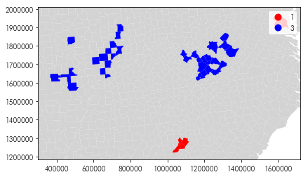
Can you focus the map in on the regions which are outliers?
f = plt.figure(figsize=(10,4))
ax = plt.gca()
ax.set_aspect('equal')
is_weird = lmos.p_sim <= (.05/len(pres))
pres.assign(quads=lmos.q)[is_weird].plot('quads',
                                         legend=True,
                                         k=4, categorical='True',
                                         cmap='bwr_r', ax=ax)
bounds = ax.axis()
pres.plot(color='lightgrey', ax=ax, zorder=-1)
ax.axis(bounds)
Group 3 moves surprisingly strongly from Obama to Trump relative to its surroundings, and group 1 moves strongly from Obama to Hilary relative to its surroundings.
Group 4 moves surprisingly away from Trump while its area moves towards Trump. Group 2 moves surprisingly towards Trump while its area moves towards Hilary.
Relaxing the significance a bit, where do we see significant spatial outliers?
pres.assign(local_score = lmos.Is,
            pval = lmos.p_sim,
            quad = lmos.q)\
    .sort_values('local_score')\
    .query('pval < 1e-3 & local_score < 0')[['name','state_name','dem_2008','dem_2016',
                                             'local_score','pval', 'quad']]
mainly in ohio, indiana, and west virginia
What about when comparing the voting behavior from 2012 to 2016?
np.random.seed(21)
lmos16 = esda.moran.Moran_Local(pres.swing_2016, w,
                              permutations=70000) #min for a bonf. bound
(lmos16.p_sim <= (.05/len(pres))).sum()
pres.assign(local_score = lmos16.Is,
            pval = lmos16.p_sim,
            quad = lmos16.q)\
    .sort_values('local_score')\
    .query('pval < 1e-3 & local_score < 0')[['name','state_name','dem_2008','dem_2016',
                                             'local_score','pval', 'quad']]
What is the relationship between the Gini coefficient and partisan swing?
sns.regplot(pres.gini_2015,
            pres.swing_full)
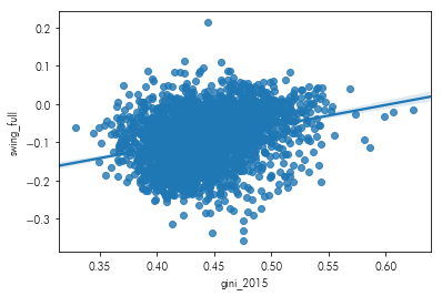
Hillary tended to do better than Obama in counties with higher income inequality. In contrast, Trump fared better in counties with lower income inequality. If you’re further interested in the sometimes-counterintuitive relationship between income, voting, & geographic context, check out Gelman’s Red State, Blue State.
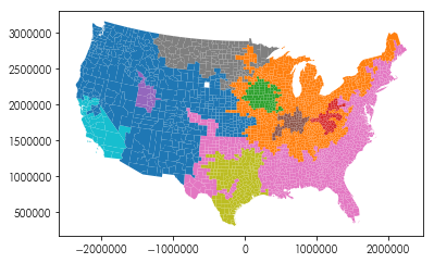
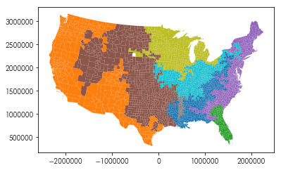
Find 8 geographical regions in the US two-party vote since 2008
from sklearn import cluster
clusterer = cluster.AgglomerativeClustering(n_clusters=8, connectivity=w.sparse)
clusterer.fit(pres.filter(like='dem_').values)
pres.assign(cluster = clusterer.labels_).plot('cluster', categorical='True')
Find 10 geographical clusters in the change in US presidential two-party vote since 2008
clusterer = cluster.AgglomerativeClustering(n_clusters=10, connectivity=w.sparse)
clusterer.fit(pres.filter(like='swing_').values)
pres.assign(cluster = clusterer.labels_).plot('cluster', categorical='True')