Topics in Working with Spatial Data
Below, we’ll take you through a typical workflow with spatial data, including some of the tricker or more difficult parts of cleaning, aligning, and cross-referencing between datasets. We’ll cover a few topics:
- creating geographic data from flat text
- geocoding to create geographic data using
geopy - creating better maps with basemaps using
contextily - building zones for visualization
- spatial joins, & queries
First, though, we’ll be mainly using the following packages:
import geopandas # to read/write spatial data
import matplotlib.pyplot as plt # to visualize data
import pandas # to read/write plain tables

# to display a few webpages within the notebook
from IPython.display import IFrame
%matplotlib inline
Reading data
In many of the “clean” analysis cases, an analyst will have prepared data that is ready to use for spatial analysis. This may mean it comes in a variety of well-understood geographical formats (e.g. shapefiles, tiff rasters, geopackage .gpkg files, or geojson). However, it is important to understand how to create geodata from flat text files, since this is a common issue when working with databases or non-specialist databases.
Below, we will read in some data from insideairbnb.com, with data pertaining to the features & prices of airbnbs in Austin, TX. This data mimicks two common ways that geographical data is distributed, when it is distributed outside of an explicitly spatial format.
neighborhoods = pandas.read_csv('../data/neighborhoods.csv')
listings = pandas.read_csv('../data/listings.csv.gz')
For the first dataset, the listings data, records are provided with information about the latitude & longitude of the listing:
listings.head()
We can see that there are multiple distinct pieces of usable geographic information in the list of columns in the dataframe:
- city
- state
- zipcode
- hood, which means neighborhood
- country
- latitude & longitude, which are the coordinates of the listing
- geometry, which is the well-known text representation of the point iself.
We will focus on constructing geometries from the latitude & longitude fields.
list(listings.columns)
Inspecting the second dataset, we can see only one column that might be relevant to constructing a geographical representation of the data. There, wkb refers to a well-known binary representation of the data. This is a common format for expressing geometric information, especially when working with spatial databases like postgis, or when geographic information is “shoehorned” into existing flat-text file formats. Often, the well-known binary representation is a string of binary digits, encoded in hexidecimal, that represents the structure of the geometry corresponding to that record in the dataframe. Neighborhoods are “areal” features, meaning that they are polygons. Thus, the well-known binary column encodes the shape of these polygons.
neighborhoods.head()
Creating geometries from raw coordinates
For the first dataset, geopandas has helper functions to construct a “geodataframe”, a subclass of pandas dataframe useful for working with geographic data, directly from coordinates. You can do this yourself using the points_from_xy function:
geometries = geopandas.points_from_xy(listings.longitude, listings.latitude)
Then, sending these geometries to the GeoDataFrame constructor, you can make a geodataframe:
listings = geopandas.GeoDataFrame(listings, geometry=geometries)
For the neighborhoods data, we must parse the well-known binary. The package that handles geometric data in Python is called shapely. Using the wkb module in shapely, we can parse the well-known binary and obtain a geometric representation for the neighborhoods:
from shapely import wkb
neighborhoods['geometry'] = neighborhoods.wkb.apply(lambda shape: wkb.loads(shape, hex=True))
neighborhoods.geometry[0]

However, even though we have parsed the geometry information, we have not ensured that this data is contained within a GeoDataFrame. Fortunately, we can use the GeoDataFrame constructor, which will use whatever is in the column called 'geometry' as the geometry for the record, by default:
neighborhoods = geopandas.GeoDataFrame(neighborhoods)
neighborhoods.drop('wkb', axis=1, inplace=True)
Writing out to file
Since it will be handy to use this data later, we will write it out to an explicit geographic data format. For now, the recommended standard in the field is the geopackage, although many folks use other data formats.
Before we can proceed, however, we need to define a coordinate reference system for the data. This refers to the system that links the coordinates for the geometries in our database to locations on the real earth, which is not flat. Inspecting our data a little bit, we can see that the coordinates appear to be in raw longitude/latitude values:
listings.geometry[[0]]
neighborhoods.geometry[[0]]
The typical coordinate reference system for data in raw latitude/longitude values is epsg:4326. To set the “initial” coordinate system for a geodataframe, the following convention is used:
neighborhoods.crs = {'init': 'epsg:4326'}
listings.crs = {'init':'epsg:4326'}
Then, we can write them out to file using the to_file method on a geodataframe:
neighborhoods.to_file('../data/neighborhoods.gpkg', driver='GPKG')
listings.to_file('../data/listings.gpkg', driver='GPKG')
Finding Addresses
It’s often important to be able to identify the address of a given coordiante, and to identify the coordinates that apply to a given address. To get this information, you can use a geocoder to work “forward,” giving the coordinates that pertain to a given address, or “backward,” giving the address pertaining to a given coordinate. Below, we’ll show you how to use geopy to do both directions of geocoding.
import geopy
The geopy package requires that you first build a “coding” object, then use that coding object to code locations. Coding forward is handled by the geocode method, and coding backwards is handled using the reverse method.
According to the terms of service, you must always set the user_agent argument when using Nominatim, the Open Street Map geocoder. geopy exposes many other geocoders for simple use, but Nominatim is the simplest to work with when getting started, because it does not require an API key, and works alright for light, occasional use.
coder = geopy.Nominatim(user_agent='scipy2019-intermediate-gds')
The reverse coding method takes a coordinate pair (in (latitude,longitude) form!) and returns a Location object, which contains quite a few handy bits of information about the query location. This includes a street address, as well as the raw data from the Nominatim API:
coder.reverse?
address = coder.reverse((listings.latitude[0], listings.longitude[0]))
address
address.raw
Since it is often the case we just want the address, we might reverse geocode the first twenty Airbnb listings from their latitude and longitude using the following apply statement:
listings.head(20)[['latitude', 'longitude']]\
        .apply(lambda coord: coder.reverse(coord).address, axis=1)
Working in the other direction, the geocode method takes a known address and converts it into a location. Using our earlier geocoded address, this works like this:
coder.geocode(address.address)
Be careful of the usage policy for the Nomiantim browser, however. There are some constraints on how Nominatim may be used. If you plan on geocoding extensively, definitely be sure to register for another service; you will get banned from using Nominatim if you send large batches of bulk geocoding requests:
IFrame('https://operations.osmfoundation.org/policies/nominatim/', width=800, height=800)
Take the next 5 minutes to try geocoding /reverse geocoding a few addresses/coordinates.
Cleaning Data
As is often the case, data never arrives perfectly clean. Later, we’ll be examining the information on the nightly price per head for Airbnbs. So, let’s take a look at how clean the price data actually is:
listings.price.head()
Ok! The price data’s dtype is object, meaning that each record is a string. The data is expressed using conventional North American price string formats, like:
$1,234.56
Which we must process into the pythonic representation of a number string:
1_234.56
To do this, we can use string methods of the price column. The .str attribute for pandas.Series objects lets us refer to string methods (like .replace(), .startswith(), or .lower()) that will be applied to every element within that Series. Since these are standard methods, they can be chained together in a sequence, as well. So, to convert our prices, we can do the following:
listings['price'] = (listings.price.str.replace('$','') # replace dollars with nothing
                                  .str.replace(',','_') # swap , for _
                                  .replace('', pandas.np.nan) # an empty string is missing data
                                  .astype(float)) # and cast to a float
Now, the price column is a float:
listings.price.head()
and can be worked with like a float:
listings.price.hist(bins=300)
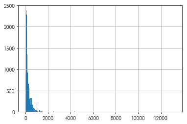
Woah,
what Airbnb costs up there at around 14k dollars/night?
listings.iloc[listings.price.idxmax()][['id','name','price', 'accommodates','listing_url']]
Taking a look at this listing, we see that it’s a huge space:
IFrame(src=listings.iloc[listings.price.idxmax()].listing_url,
       width=800, height=800)
Further, quite a few prices are down at zero dollars! That’s… odd! For now, let’s drop values that have extremely low and high prices.
listings = listings[listings.price < listings.price.quantile(.99)]
listings = listings[listings.price > listings.price.quantile(.01)]
Basemaps
Basemaps are visual aids that sit below your data that help to contextualize information being displayed on a map. We suggest using the contextily package alongside geopandas to make great, high-quality maps from web tiles. To use contextily, we must first reproject our data into the Web Mercator projection, which is used for most web mapping tiles.
listings = listings.to_crs(epsg=3857)
neighborhoods = neighborhoods.to_crs(epsg=3857)
The main functionality of contextily is contained within the bounds2img function. This function takes the bounds of a given area and returns all web tiles that intersect this area at a given zoom level. Thus, you can define a level of detail (zoom), and contextily will grab the tiles that intersect the area and return them as a numpy array.
To make this easy with geopandas, we can use the total_bounds attribute of our GeoDataFrames. This reflects the bounding box for the geometries inside of that GeoDataFrame. It is updated when data in the dataframe is changed, including when the dataframe is subsetted or appened to, so the total_bounds is an accurate reflection of the full extent of the data. Since we have transformed our data to the Web Mercator projection, the total_bounds for the data now expresses locations in terms of coordiantes within the Web Mercator system:
neighborhoods.total_bounds
Data in the total_bounds attribute is stored in (west, south, east, north) format typical of geospatial applications. In concept, this provides the lower left and top right corners of the map. For many imaging applications, such as in matplotlib, bounding box information is often given instead as (west, east, south, north), so attention must be paid to the format of these bounding boxes.
Since contextily uses the same format for bounding boxes as geopandas, you can provide the total_bounds coordinates to the constructor using the unpack operator, *:
import contextily
basemap, basemap_extent = contextily.bounds2img(*neighborhoods.total_bounds,
                                                zoom=10)
Thus, two objects are returned. basemap is a numpy raster containing the actual color values for the basemap:
basemap
The basemap_extent object contains the bounding box information for this image, encoded in Web Mercator coordinates in (west, east, south, north) form:
basemap_extent
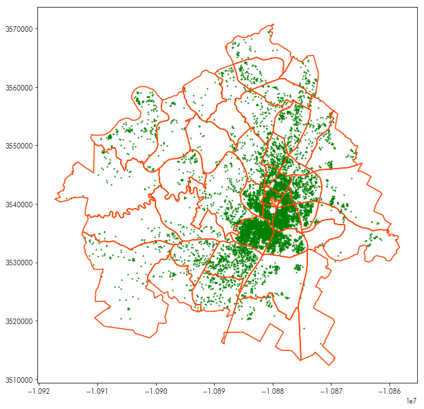
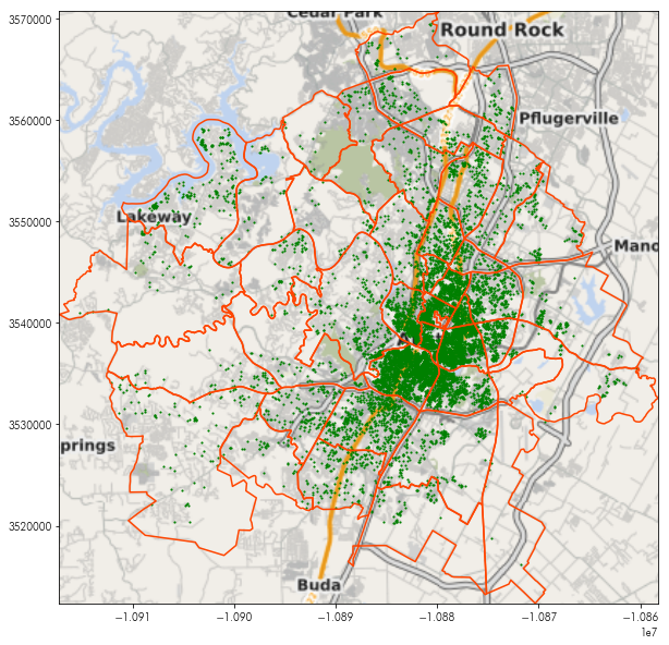
This can be used with the plt.imshow function (which displays images from numpy arrays), to provide a basemap to any plot. For example, the following plot shows the neighborhoods and listing data together:
plt.figure(figsize=(10, 10))
neighborhoods.boundary.plot(ax=plt.gca(), color='orangered')
listings.plot(ax=plt.gca(), marker='.', markersize=5, color='green')
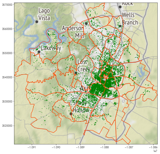
By adding the basemap in using plt.imshow, we can see where these points and polygons are:
plt.figure(figsize=(10, 10))
plt.imshow(basemap, extent=basemap_extent, interpolation='bilinear')
neighborhoods.boundary.plot(ax=plt.gca(), color='orangered')
listings.plot(ax=plt.gca(), marker='.', markersize=5, color='green')

# and, to make sure the view is focused only on our data:
plt.axis(neighborhoods.total_bounds[[0,2,1,3]])
Contextily offers many different styles of basemap. Within the contextily.tile_providers module, different providers are stated, such as:
ST_*, the family of Stamen map tilesOSM_*, the family of Open Street Map map tiles.
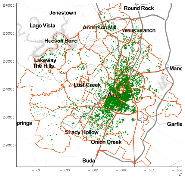
For instance, the following will show the very pretty Stamen Toner Light tiles:
tonermap, tonermap_extent = contextily.bounds2img(*neighborhoods.total_bounds, zoom=10,
                                                  url=contextily.tile_providers.ST_TONER_LITE)
plt.figure(figsize=(10,10))
plt.imshow(tonermap, extent=tonermap_extent)
neighborhoods.boundary.plot(ax=plt.gca(), color='orangered')
listings.plot(ax=plt.gca(), marker='.', markersize=5, color='green')
plt.axis(neighborhoods.total_bounds[[0,2,1,3]])
If you’re interested or able to use others’ tileservers, you can also format your tileserver query using tileZ (for zoom) and tileX/tileY, like other tileserver url formats and provide this URL to the bounds2img function:
transit = 'http://tile.memomaps.de/tilegen/tileZ/tileX/tileY.png'
transitmap, transitmap_extent = contextily.bounds2img(*neighborhoods.total_bounds, zoom=10,
                                                      url=transit)
plt.figure(figsize=(10,10))
plt.imshow(transitmap, extent=transitmap_extent, interpolation='bilinear')
neighborhoods.boundary.plot(ax=plt.gca(), color='orangered')
listings.plot(ax=plt.gca(), marker='.', markersize=5, color='green')
plt.axis(neighborhoods.total_bounds[[0,2,1,3]])
Using geopy & contextily, put together a map of your hometown, place of residence, or place of work.
hint: the bounding box of a geopy query is often contained in its raw attribute
Building up areas for visualization
Building areas for the visualization of spatial groups is a very useful tool. In many contexts, these areas provide a simple way to classify new data into groups, or can provide a simpler graphical frame with which large amounts of data can be visualized.
For our puposes, Airbnb data contains a lot of information about neighborhoods. But, people often disagree about the naming and boundaries of their neighborhoods. From a practical perspective, our data on Airbnbs has a few different pieces of information about neighborhoods. In the listings dataframe, each individual Airbnb offers up some information about what “neighborhood” it falls within:
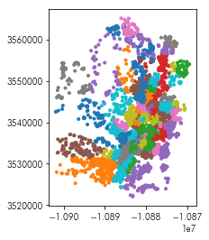
listings.dropna(subset=['hood']).plot('hood', marker='.')
Indeed, there are many different neighborhoods in the data:
(listings.groupby('hood') #group by the neighborhood
         .id.count() # get the count of observations
         .sort_values(ascending=False) # sort the counts to have the most populous first
         .head(20)) # and get the top 20
One method that is used often to construct an area from point data is to consider the convex hull of the data. The convex hull is like the polygon you’d get if you took a rubber band and stretched it around the most extreme points. Every point is inside of the convex hull, but some points will be on its boundary. Further, the shape is convex, meaning that the straight line between any two points will also be contained within the convex hull. We can build convex hulls from a group of points using the unary_union attribute of a GeoSeries (to collect them together into a single geometry), and then using the convex_hull method for that shape. For example
listings.iloc[[0,1,2,3]].geometry
listings.iloc[[0,1,2,3]].geometry.unary_union

listings.iloc[[0,1,2,3]].geometry.unary_union.convex_hull

Since this unary_union is a property of any GeoSeries and convex_hull is a property of any shapely geometry, we can use this approach within a groupby as a part of a typical split-apply-combine pattern. For instance, if we wanted to get the convex hulls for each neighborhood, we might first group by neighborhoods:
hood_groups = listings.groupby('hood')
Then, for each group, we’d want to do the same thing we did above: get the unary_union.convex_hull from that chunk:
chulls = hood_groups.geometry.apply(lambda hood: hood.unary_union.convex_hull)
If this worked, we will see each neighborhood next to a polygon corresponding to its convex hull:
chulls.head()
It did work! All that is needed now is to build a GeoDataFrame from these hulls for further analysis & mapping:
chulls = geopandas.GeoDataFrame(chulls.reset_index())
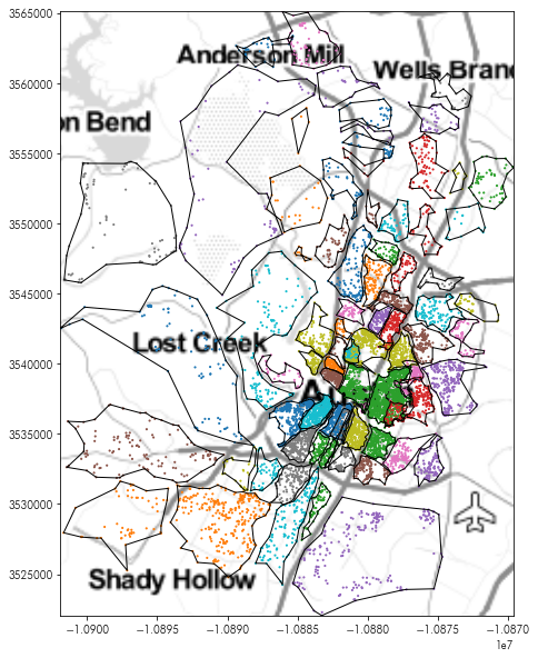
Since these convex hulls are now a standard geodataframe, we can make a map using them, just like we did the neighborhoods before:
plt.figure(figsize=(10,10))
plt.imshow(tonermap, extent=tonermap_extent, interpolation='bilinear')
chulls.boundary.plot(linewidth=1, color='k', ax=plt.gca())
listings.dropna(subset=['hood']).plot('hood', ax=plt.gca(),
                                      marker='.', markersize=5)
plt.axis(chulls.total_bounds[[0,2,1,3]])
plt.show()
Hmm…
There are some weird overlaps there:
plt.figure(figsize=(10,10))
plt.imshow(tonermap, extent=tonermap_extent, interpolation='bilinear')
chulls.boundary.plot(ax=plt.gca(), linewidth=1, color='k')
listings.dropna(subset=['hood']).plot('hood', ax=plt.gca(),
                                      marker='.', markersize=50)
plt.axis(chulls.query('hood == "Westlake Hills"').total_bounds[[0,2,1,3]])
plt.show()
The convex hull of the larger set of points can’t help but be too large; it’s shape is intrinsically not convex! The indentation where the other smaller group of points fall simply cannot be accommodated using the convex hull.
Another common kind of hull for analysis purposes is the alpha shape. Alpha shapes reflect a kind of non-convex optimally-tight hull that can be used to analyze groups of points. One implementation of this algorithm is in the Python Spatial Analysis Library, pysal. It takes an array of coordinates and returns the polygon corresponding to the Alpha Shape
from pysal.lib.cg import alpha_shape_auto
from pysal.lib.weights.distance import get_points_array
Thus, like before, we can get the coordinates from each group and compute the alpha shape for the coordinates. We do this in a similar fashion to how the convex hulls were built:
ashapes = hood_groups.geometry.apply(lambda hood: alpha_shape_auto(
                                                  get_points_array(hood)))
ashapes = geopandas.GeoDataFrame(ashapes.reset_index())
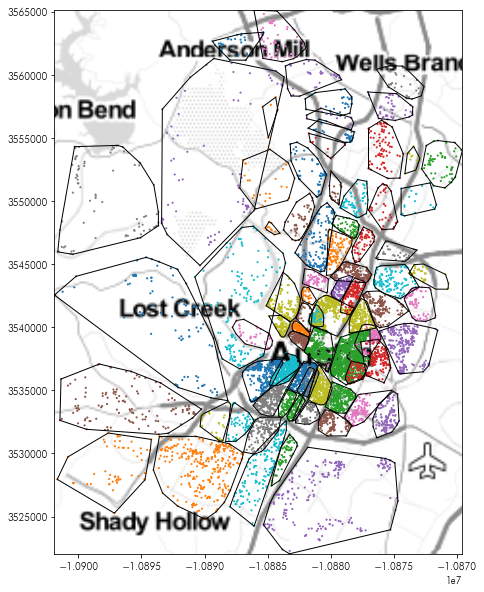
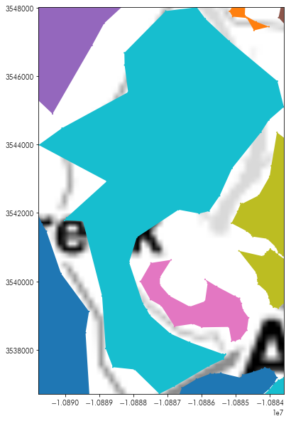
These new boundaries are no longer forced to be convex, and can be incredibly non-convex:
plt.figure(figsize=(10,10))
plt.imshow(tonermap, extent=tonermap_extent, interpolation='bilinear')
ashapes.boundary.plot(color='k', linewidth=1, ax=plt.gca())
listings.dropna(subset=['hood']).plot('hood', ax=plt.gca(),
                                      marker='.', markersize=5)
plt.axis(ashapes.total_bounds[[0,2,1,3]])
plt.show()
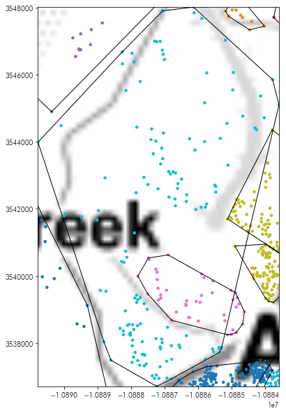
So, the overlap seen earlier does not show up:
plt.figure(figsize=(10,10))
plt.imshow(tonermap, extent=tonermap_extent, interpolation='bilinear')
ashapes.plot('hood', ax=plt.gca(), linewidth=2)
listings.dropna(subset=['hood']).plot('hood', ax=plt.gca(),
                                      marker='.', markersize=5)
plt.axis(ashapes.query('hood == "Westlake Hills"').total_bounds[[0,2,1,3]])
plt.show()
Spatial Joins
But, we have the neighborhoods data as well. How do these relate to the neighborhoods we’ve just built?
plt.figure(figsize=(10,10))
plt.imshow(tonermap, extent=tonermap_extent, interpolation='bilinear')
ashapes.plot(linewidth=1, ax=plt.gca())
neighborhoods.plot(ax=plt.gca(), alpha=.5,
                   edgecolor='red', facecolor='lightyellow')
plt.axis(ashapes.total_bounds[[0,2,1,3]])
plt.show()
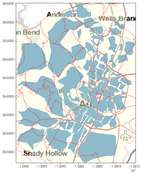
It looks like there are many neighborhoods where the neighborhood stated in the listing isn’t the neighborhood provided by the insideairbnb project. To see how the two relate to one another, we can use a spatial join.
Spatial joins are used to relate recrods in a spatial database. To join two spatial tables together using a spatial join, you first need to think of what the spatial query is that is answered by the spatial join. Common spatial queries that are answered by spatial joins might be:
- How many fire stations are within each residential district?
- Which rivers flow under a street?
- What is the most common political yard sign on each street segment?
In each of these cases, we’re seeking to answer a question about the relationship between two spatial datasets. In the first, we’re asking how many fire stations (a point- or a polygon-based geometry) fall within a residential district (a polygon-based geometry). In the second, we’re asking how many rivers (a line- or a polygon-based geometry) flow underneath a street (a line- or polygon-based geometry). In the last, we are asking what the most common yard sign (a point-based geometry) on each street segment (a line-based geometry). The spatial relationshps used for each of these queries would depend on the order used in the join. For instance, fire stations within residential districts would indicate a within relation, but reversing the spatial relationship yields a valid query as well residential districts contain fire stations. Formally speaking, the spatial relationships considered by spatial joins are defined formally by the Dimensionally-Extended 9-Intersection Model, but most common joins are stated in terms of one of three operations:
- A intersects B: the final table contains records that unite the features of A and B for each pair of observations whose geometries intersect in any manner.
- A contains B: the final table contains records that unite the features of A and B for each pair of observations where the record in A “contains”, or fully covers, the record in B
- A is within B: the final table contains records that unite the features of A and B for each pair of observations where the record in A is within a record of B
When feature a contains feature b, then feature b is within feature a. These can be thought of as the inverse relations of one another.
For us to discover which listings are within each neighborhood, we can specify the within op (short for operation) in the geopanda.sjoin function:
listings_in_hoods = geopandas.sjoin(listings, neighborhoods, op='within')
In total, there are three relations supported by geopandas.
- Intersects: a record from the left table intersects a record from the left table.
- Within: a record from the left table is within a record from the right table.
- Contains: a record from the left table contains a record from the right table.
The result from a spatial join creates a table where each row combines the left and right dataframes when the spatial operation is True. We can see that the index and hood_id from the neighborhoods table is brought alongside the id and hood data from the listing table:
listings_in_hoods.head()[['id', 'hood', 'index_right', 'hood_id']]
In this new joint table, we can count the different neighborhoods from the listing table that fall within each neighborhood from the neighborhood table:
compositions = listings_in_hoods.groupby(('hood', 'hood_id')).id.count()
compositions
To reformat this in a manner that can be easier to use, we can restate it in terms of the square join matrix by unstacking it and replacing the NaN values with something easier on the eyes, like a ‘-‘ string:
compositions.unstack().fillna('-')
From here, we could make a map of the number of neighborhoods that listings say they are in veruss the neighborhoods Airbnb uses internally. To do this, we would need to get the number of neighborhood names from the listings table that occur within each neighborhood from the neighborhood table.
To do this, we might first group the spatially-joined table listings_in_hoods by the hood_id (from the neighborhood table) and get the unique hood names (from the listing table) that occur in that group:
listings_in_hoods.dropna(subset=['hood']).groupby('hood_id').hood.unique()
The length of this list of unique names is the length of unique hood names within each neighborhood from the neighborhood dataframe:
number_unique = listings_in_hoods.dropna(subset=['hood']).groupby('hood_id')\
                                 .hood.unique().apply(len)
number_unique.head()
Then, to merge this back into the neighborhoods frame, we can use a typical aspatial table merge:
saidhoods_in_hood = neighborhoods.merge(number_unique.to_frame('number_names'),
                                        how='left',
                                        left_on='hood_id', right_index=True)
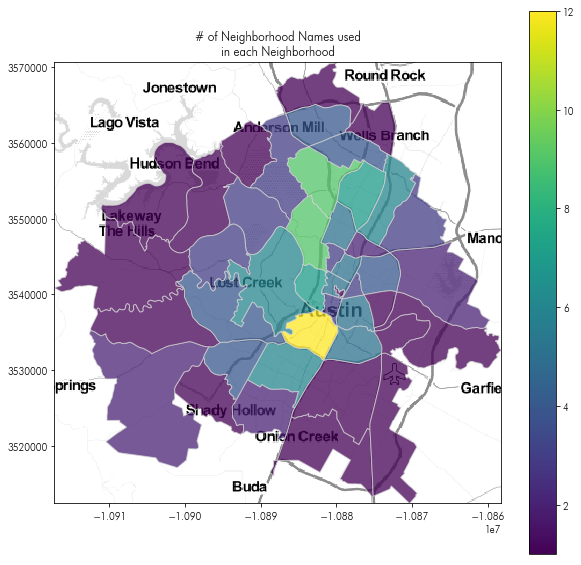
And (finally) make a map of the number of neighborhood names that hosts say within each neighborhood Airbnb uses for analytics:
plt.figure(figsize=(10,10))
plt.imshow(tonermap, extent=tonermap_extent)
saidhoods_in_hood.plot('number_names', ax = plt.gca(),
                       alpha=.75, edgecolor='lightgrey', legend=True)
plt.title('# of Neighborhood Names used\nin each Neighborhood')
plt.axis(saidhoods_in_hood.total_bounds[[0,2,1,3]])
What do nearby airbnbs look like?
Another kind of spatial “join” focuses on merging two datasets together by their proximity, rather than by one of the spatial relations discussed above. These queries often are used to ask questions like:
- What is the nearest restaurant to my hotel?
- How many bars are within a 20-minute walk of the conference center?
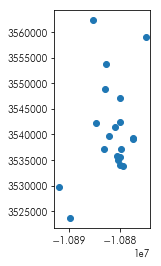
This distance-based query can occasionally be answered focusing explicitly on DE-9IM-style queries like we discussed above. For instance, response 2 can be answered using a buffer. In spatial analysis, a buffer is the polygon developed by extending the boundary of a feaure by a pre-specified distance. For example, given the points below:
listings.head(20).plot()
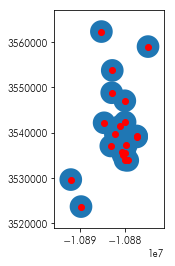
The buffer of these points would “inflate” these points into a circle of a specified distance:
ax = listings.head(20).buffer(2500).plot()
listings.head(20).plot(ax=ax, color='red')
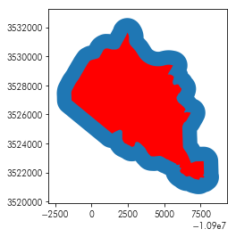
For a polygon or line, a buffer works similarly:
ax = neighborhoods.iloc[[0]].buffer(1000).plot()
neighborhoods.iloc[[0]].plot(color='red', ax=ax)
As such, a query like
what is the average price per head in 1000 meters around each Airbnb
can be reframed in terms of a spatial join between the 1000 meter buffer around each airbnb and the original Airbnbs themselves. To do this for Airbnbs in Downtown Austin, we could do the following few steps.
First, we can pick the two downtown neighborhoods in our dataset:
downtown_hoods = ('Downtown', 'East Downtown')
And then, using the standard pandas DataFrame.query functionality, focus the analysis on only the neighborhoods in the downtown:
downtown_listings = listings.query('hood in @downtown_hoods')
Then, we can build a buffer around each Airbnb using the buffer method:
searchbuffer = downtown_listings.buffer(1000)
This returns a GeoSeries, the geopandas analogue of the pandas.Series.
searchbuffer.head()
We can use this to build a dataframe where the values are the price per head at each airbnb, and the geometry is the buffer. We’ll keep the id from the downtown_listings dataframe as well.
searchbuffer = geopandas.GeoDataFrame(downtown_listings.price.values/downtown_listings.accommodates.values,
                                      geometry=searchbuffer.tolist(),
                                      columns=['buffer_pph'],
                                      index=downtown_listings.id.values)
searchbuffer.crs = downtown_listings.crs
searchbuffer.head()
Then, we can compute the average price within 1000 meters of each Airbnb by finding which 1000 meter buffers intersect each Airbnb listing:
listing_buffer_join = geopandas.sjoin(downtown_listings, searchbuffer, op='intersects')
However, we want to ensure that there are no “self-joins.” Since a buffer of 1000 meters around a point intersects the point itself, we must remove self-joins from the final query. Since we indexed the searchbuffer frame using the id field, we can drop all entries where id == index_right.
listing_buffer_join = listing_buffer_join.query('id != index_right')
Now, each record in listing_buffer_join describes the relationship between an Airbnb and a 1-km buffer around a different Airbnb. By grouping together all records with the same id, we can summarize the prices of the nearby buffers.
downtown_areasummaries = listing_buffer_join.groupby('id').buffer_pph.describe()
For an indication of what this looks like, we can look at the head of the dataframe:
downtown_areasummaries.head()
There, there are 222 other Airbnbs within a single kilometer of listing 2265, and the average price per head of those listings is \$57.53 dollars per night.
To link this back up with the original data, we can merge the downtown_areasummaries back up with the downtown_listings since they both share the listing id:
downtown_areasummaries = downtown_listings.merge(left_on='id',
                                                 right=downtown_areasummaries,
                                                 right_index=True, how='left')
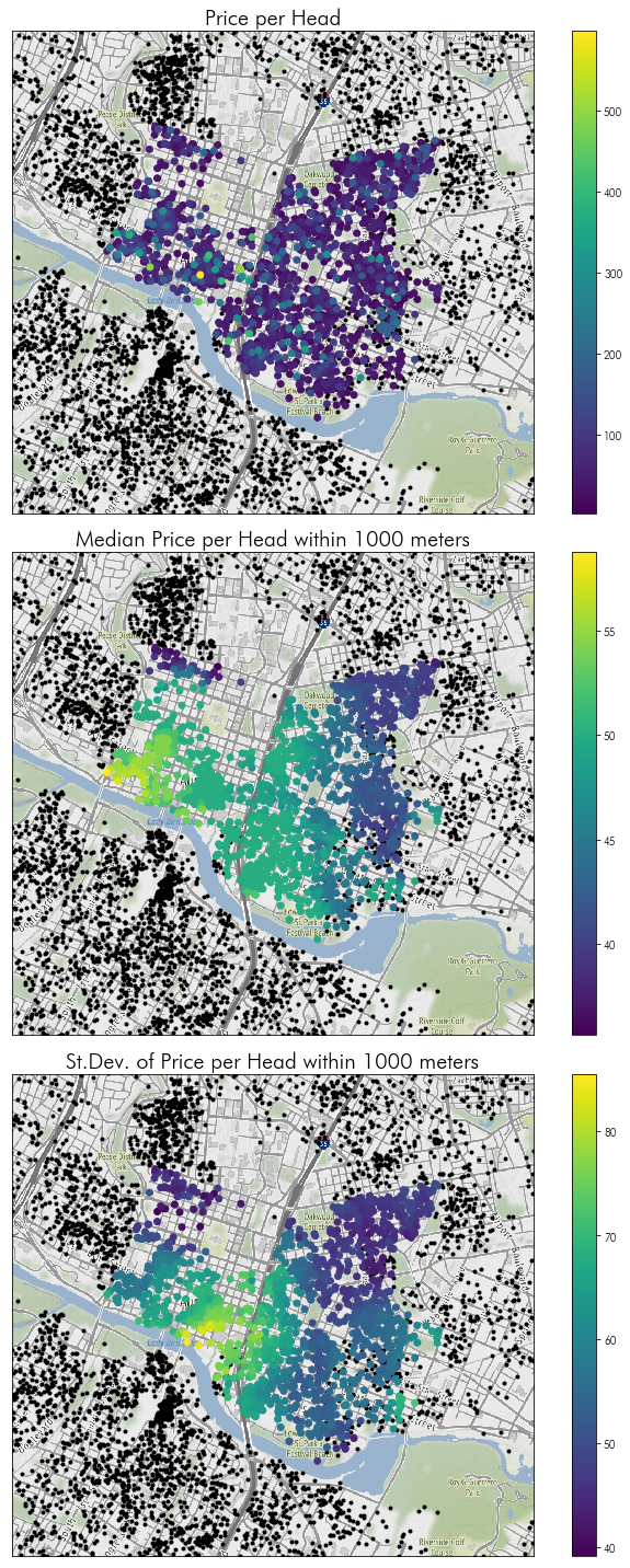
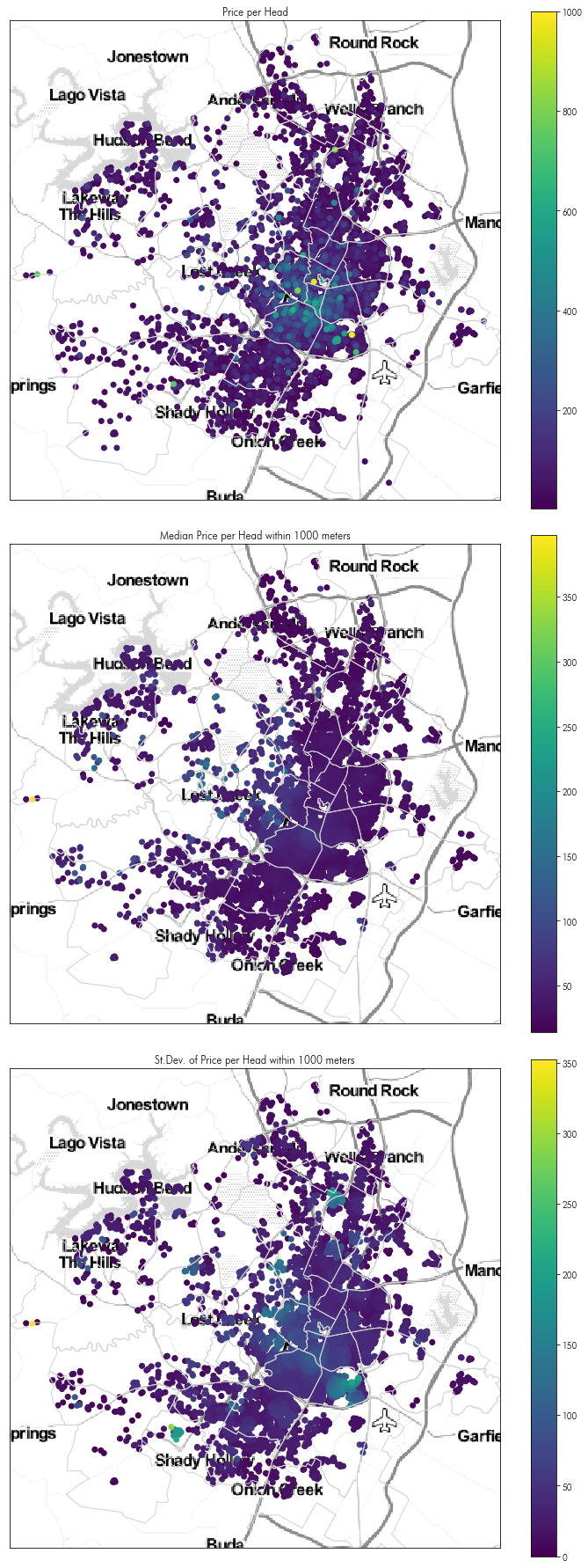
Then, we can plot these “surrounding characteristics”, showing the spatially-smoothed average of prices in the downtown Austin area:
f, ax = plt.subplots(3,1,figsize=(10,20), sharex=True, sharey=True)
downtown_basemap, downtown_basemap_extent = contextily.bounds2img(*downtown_listings.buffer(1500).total_bounds, zoom=14)
for ax_ in ax:
    listings.plot(color='k', marker='.', ax=ax_)
    ax_.set_xticks([])
    ax_.set_xticklabels([])
    ax_.set_yticks([])
    ax_.set_yticklabels([])
    ax_.imshow(downtown_basemap, extent=downtown_basemap_extent)

downtown_listings.eval('price_per_head = price / accommodates')\
                 .sort_values('price_per_head', ascending=True)\
                 .plot('price_per_head',
                       ax=ax[0], legend=True)

downtown_areasummaries.sort_values('50%', ascending=True)\
        .plot('50%', ax=ax[1], legend=True)
downtown_areasummaries.sort_values('50%', ascending=True)\
        .plot('std', ax=ax[2], legend=True)


ax[1].axis(listings.query('hood in @downtown_hoods').total_bounds[[0,2,1,3]])
ax[0].set_title('Price per Head', fontsize=20)
ax[1].set_title('Median Price per Head within 1000 meters', fontsize=20)
ax[2].set_title('St.Dev. of Price per Head within 1000 meters', fontsize=20)
ax[0].axis(downtown_listings.buffer(1500).total_bounds[[0,2,1,3]])

f.tight_layout()
Moving beyond a toy problem…
this gets difficult to process. The join between the buffer polygons and the listings becomes very computationally intensive, even when spatial indices are used. Therefore, it can be easier, especially when dealing with point queries, to use a K-D Tree. These are special data structures (provided by scipy) that allow for exactly these kinds of queries. A useful helper function as well is provided by pysal, namely the get_points_array function. This function extracts the coordinates of all vertices for a variety of geometry packages in Python and returns a numpy array.
from pysal.lib.weights.distance import get_points_array
import numpy
To do this distance-based price join for the whole map, then, we need to extract the coordinates and the prices of all the Airbnb listings:
coordinates = get_points_array(listings.geometry)
prices = listings.price.values / listings.accommodates.values
Then, we must build the KDTree using scipy. For nearly any application, the cKDTree will be faster. KDTree is an implementation of the datastructure in pure Python, whereas the cKDTree is an implementation in Cython.
from scipy.spatial import cKDTree
KDTrees are objects. We will tend to use the query_* methods from the KDTree. KDTrees in scipy are built when instantiated, and typically the instantiation is an expensive enough computation for large datasets that you will want to avoid re-computing the tree itself if you plan to query from it multiple times.
kdt = cKDTree(coordinates)
There are many query_* functions on the KDTree. We will use the query_ball_tree function to do the same thing as we did above:
kdt.query_ball_tree?
neighbors = kdt.query_ball_tree(kdt, 1000)
The query_ball_tree function returns a list of lists, where the $i$th list indicates the set of neighbors to the $i$th observation that are closer than $r$ to $i$.
numpy.asarray(neighbors[0])
To summarize this in the same fashion we did before, we must again remove self-neighbors. There are many ways to optimize this, since it is both embarassingly parallel and can be forced to work with arrays, but we opt for simplicity in using this generator below:
neighbors = ([other for other in i_neighbors if other != i] for i,i_neighbors in enumerate(neighbors))
Then, to get the same information as above (the median & standard deviation of prices for nearby Airbnbs), we can use the following summary helper function:
def summarize(ary):
    return numpy.median(ary), numpy.std(ary)
and compute the summary of the prices at each neighbor:
summary = numpy.asarray([summarize(prices[neighbs]) for neighbs in neighbors])
Since the input data is in the same order as the listings dataframe, we can assign directly back to the original dataframe:
medians, deviations = zip(*summary)
listings['median_pph_1km'], listings['std_pph_1km'] = medians, deviations
And we can make a similar sort of map as to that focusing on Downtown above, but for the whole of Austin:
f, ax = plt.subplots(3,1,figsize=(10,25), sharex=True, sharey=True)

listings.eval('price_per_head = price / accommodates')\
        .sort_values('price_per_head', ascending=True)\
        .plot('price_per_head', ax=ax[0], legend=True)

listings.sort_values('median_pph_1km', ascending=True)\
        .plot('median_pph_1km', ax=ax[1], legend=True)
listings.sort_values('std_pph_1km', ascending=True)\
        .plot('std_pph_1km', ax=ax[2], legend=True)


ax[0].set_title('Price per Head')
ax[1].set_title('Median Price per Head within 1000 meters')
ax[2].set_title('St.Dev. of Price per Head within 1000 meters')

for ax_ in ax:
    ax_.set_xticks([])
    ax_.set_xticklabels([])
    ax_.set_yticks([])
    ax_.set_yticklabels([])
    ax_.imshow(tonermap, extent=tonermap_extent)
    ax_.axis(listings.buffer(2000).total_bounds[[0,2,1,3]])
    neighborhoods.plot(ax=ax_, edgecolor='lightgrey', facecolor='none')

f.tight_layout()
How about nearest neighbor joins?
The KDTree also works for queries about the properties of nearest points as well. For instance, it may be helpful to know how homogenous the types of Airbnbs are across Austin. Areas with many Airbnbs all of the same type (e.g. Entire home/apt) may be areas where the market for temporary housing is relatively homogenous in its offerings overall. Thus, we might define a distinction between Airbnbs which are fully “private” and those that involve some kind of shared component by building an indicator variable for whether or not a listing is shared in some manner:
is_shared = ~ (listings.room_type=="Entire home/apt")
Then, we can build a KDTree for each type of listing:
shared_kdt = cKDTree(coordinates[is_shared])
alone_kdt = cKDTree(coordinates[~ is_shared])
And, using the query function, find which is the nearest listing in the other group:
shared_kdt.query?
Reading that docstring, we can see that the query function returns two things in a tuple. The first is the distance from the observation on the left to the observation on the right. The second is the index of the right observation. These are always sorted by the distances, so that the nearest observation corresponds to the first distance, and the second observation to the second distance, etc.
Thus, using the query across the two groups provides the nearest entry to each observation in each group:
nearest_unshared_dist, nearest_unshared_ix = shared_kdt.query(coordinates[~is_shared], k=1)
nearest_alone_dist, nearest_alone_ix = alone_kdt.query(coordinates[is_shared], k=1)
Pause, for a moment before moving on to answer for yourself:
why can’t we just use one query?
(hint: think of each city’s nearest other city amongst LA, San Francisco, and Chicago. Is the relationship always symmetric?)
With this in mind, we can assign the two distances together into a single vector. Since the indices are positions (i.e. not names), we can convert them back to the names in the dataframe by indexing the listings.index array using their values.
listings.loc[~is_shared, 'nearest_othertype'] = listings.index[nearest_unshared_ix]
listings.loc[is_shared, 'nearest_othertype'] = listings.index[nearest_alone_ix]
Since the distances correspond directly to the indices, we can simply assign those directly:
listings.loc[~is_shared, 'nearest_othertype_dist'] = nearest_unshared_dist
listings.loc[is_shared, 'nearest_othertype_dist'] = nearest_alone_dist
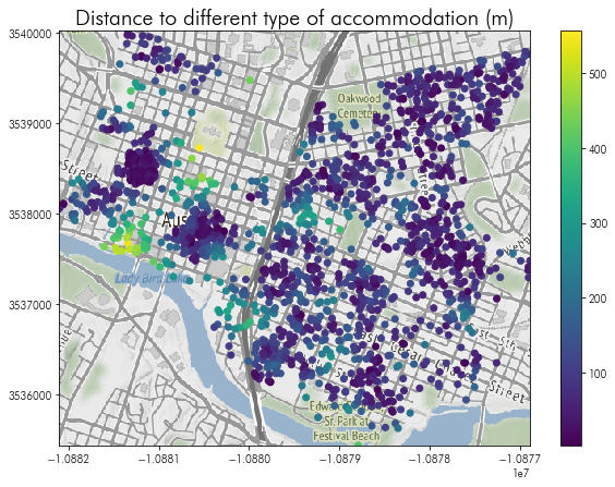
Then, we can visualize the distances to the nearest different type of accommodation, like before:
f = plt.figure(figsize=(10,7))
plt.imshow(downtown_basemap, extent=downtown_basemap_extent)
listings.query('hood in @downtown_hoods').plot('nearest_othertype_dist', ax=plt.gca(), legend=True)
plt.axis(downtown_listings.total_bounds[[0,2,1,3]])
plt.title('Distance to different type of accommodation (m)', fontsize=20)
Now, we will pause for a short break & questions before moving to the problemset, relations-problemset.ipynb.