This page was generated from notebooks/topo.ipynb. Interactive online version:

Topological Measures of Geographical Surfaces

Levi John Wolf

import warnings

import geopandas
import matplotlib.pyplot as plt
import numpy
from libpysal import weights

from esda import topo

This notebook explains the usage and meaning of the topo functions, prominence and isolation. Both of these concepts arise from topography, the study of the forms and features of a surface.

In this sense, topographical measures focus on the shape of a surface. In physical geography, prominence and isolation are both topographical measures that refer to how high (or how “dominant”) a mountain is relative to its landscape. Mathematically, if we represent “elevation” with a surface (like a Digital Elevation Model, or DEM), then this becomes a way to characterize the local maxima, minima, and/or saddle points of a given surface. In this way, prominence (and isolation) are intricately connected to the local extrema and concavity/convexity of a surface, and provide useful ways to think about the structure of a geographical distribution. In a physical sense, the isolation of a mountain peak is the distance you have to travel to find a higher point on the surface. So, the common example given, say, on Wikipedia, is that Mount Everest has an “infinite” isolation, since it is the highest point on Earth’s surface. The nearby peak K2, the second-highest mountain on Earth is relatively close to Everest, so K2 has quite a low isolation. However, Aconcauga, the tallest peak in the Western Hemisphere, is about 1,000 meters shorter than K2, but way more isolated, since the distance from it to the nearest highest point is very large. So, isolation is a measure of horizontal distance.

In contrast, prominence is a measure of vertical distance, describing the gap between the peak’s elevation and the “highest” low point between it and its parent peak. Conceptually, imagine that the whole world is flooded, all the way to the top of Mount Everest. Let’s denote the height of mountain \(i\) as \(h_i\), and the water level as \(w\). So, starting with \(max(h_i) = w\), we lower the water. When \(h_i = w\), a peak “emerges” from the water. Imagine two peaks of height \(h_i\) and \(h_j\) (such that \(h_i > h_j\)). Then, imagine that \(w\) falls to a point \(w^* < h_j < h_i\) where \(h_i\) and \(h_j\) become “connected” together as part of a single landmass. Then, the prominence of \(h_j\) is computed as \(p_j = h_i - w^*\), the relative height between peak \(j\) and the lowest point connecting \(j\) and \(i\). In this model, it makes sense to then consider \(j\) and \(i\) the same peak \((ij)\), and measure the next peak’s prominence as the lowest point between \(k\) and \((ij)\). We use prominence because it tells you how high a peak/local maxima is relative to its surroundings.

Things are complicated somewhat when we’re dealing with irregular or dis-continuous relief. When dealing with mountains and elevation, we know that elevation is a surface that changes (relatively) smoothly. In contrast, most of our vector data does not change smoothly. Despite this, we can still use these notions of isolation and prominence to measure the relative contrasts between parts of a geographcial surface.

So, for what happens next, we’ll refer to the natural earth dataset baked into geopandas. We’ll use the population estmate (pop_est) as a kind of “elevation,” a la @undertheraedar’s excellent population topography:

Isolation and Prominence of country populations

Let’s start with a natural example: isolation of population of countries.

natearth = geopandas.read_file(
    "https://naciscdn.org/naturalearth/110m/cultural/ne_110m_admin_0_countries.zip"
)

To start, we know that China, India, and the US are the three most populous countries in the world:

natearth.sort_values("POP_EST", ascending=False).head()

	featurecla	scalerank	LABELRANK	SOVEREIGNT	SOV_A3	ADM0_DIF	LEVEL	TYPE	TLC	ADMIN	...	FCLASS_TR	FCLASS_ID	FCLASS_PL	FCLASS_GR	FCLASS_IT	FCLASS_NL	FCLASS_SE	FCLASS_BD	FCLASS_UA	geometry
139	Admin-0 country	1	2	China	CH1	1	2	Country	1	China	...	None	None	None	None	None	None	None	None	None	MULTIPOLYGON (((109.47521 18.1977, 108.65521 1...
98	Admin-0 country	1	2	India	IND	0	2	Sovereign country	1	India	...	None	None	None	None	None	None	None	None	None	POLYGON ((97.32711 28.26158, 97.40256 27.88254...
4	Admin-0 country	1	2	United States of America	US1	1	2	Country	1	United States of America	...	None	None	None	None	None	None	None	None	None	MULTIPOLYGON (((-122.84 49, -120 49, -117.0312...
8	Admin-0 country	1	2	Indonesia	IDN	0	2	Sovereign country	1	Indonesia	...	None	None	None	None	None	None	None	None	None	MULTIPOLYGON (((141.00021 -2.60015, 141.01706 ...
102	Admin-0 country	1	2	Pakistan	PAK	0	2	Sovereign country	1	Pakistan	...	None	None	None	None	None	None	None	None	None	POLYGON ((77.83745 35.49401, 76.87172 34.65354...

5 rows × 169 columns

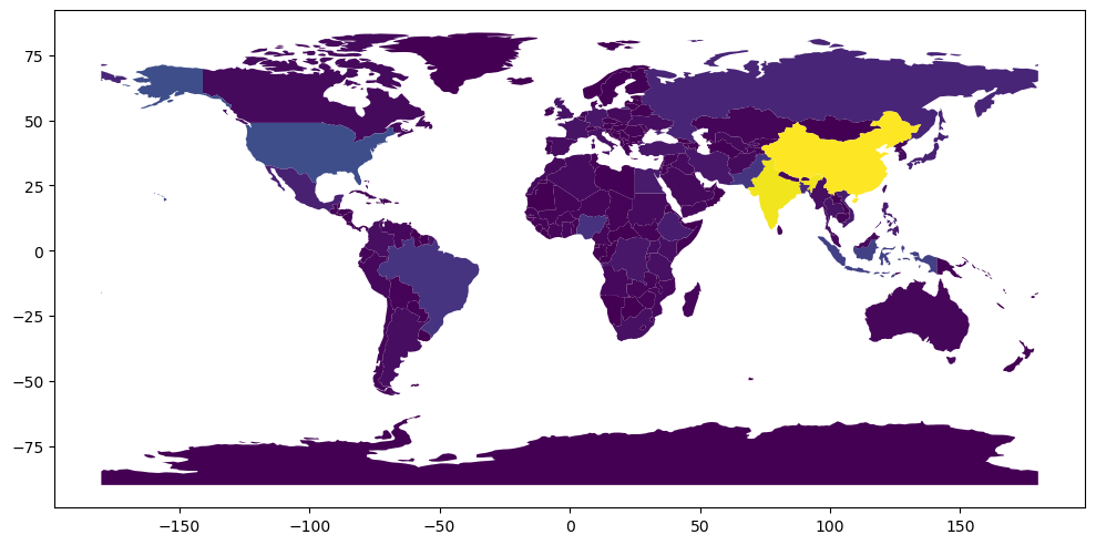
This is a perfect dataset to think about isolation/prominence, since we have big gaps between the highest population points in each continent.

f, ax = plt.subplots(1, 1, figsize=(12, 6))
natearth.plot("POP_EST", ax=ax)

<Axes: >

To simplify things, we’ll just consider the Euclidean distances between country centroids, but we could (in theory) use any kind of distance we want in this function by specifying the metric argument.

with warnings.catch_warnings():
    warnings.filterwarnings(
        "ignore",
        category=UserWarning,
        message="Geometry is in a geographic CRS",
    )

    coordinates = numpy.column_stack((natearth.centroid.x, natearth.centroid.y))

To get a bit more information on the result, we can use return_all to get the rank and distance for the isolated peak. This also returns the gap between the peak and its nearest higher peak.

iso = topo.isolation(natearth["POP_EST"], coordinates, return_all=True)

Under the hood, this algorithm uses rtree and numpy.sort to insert observations into a SpatialIndex() in rank-order. Iterating down the ranks, the nearest higher observation is found in the SpatialIndex(), and that becomes the parent of that observation. As we iterate, pop_est gets smaller and smaller, and more and more entries are added to the rtree.

Merging this back to the data we have will let us visualize it.

natearth = natearth.merge(iso, left_index=True, right_index=True)

So, you can see that the isolation for China is infinite, since there is no country with a larger population. However, the isolation for India is only the distance from China to India (27). The isolation for the US, however, is much larger, and reflects the distance from the US to India (which just happens to be closer than China). The fourth-most populous country, Indonesia, is closer to China than India, so its parent_rank is 0, and its isolation is the distance from Indonesia to China. Last, you see Brazil, 5th most populous country, has US as a parent, with an isolation distance of 82.

natearth[
    ["CONTINENT", "NAME", "rank", "POP_EST", "parent_rank", "isolation", "gap"]
].sort_values("POP_EST", ascending=False).head()

	CONTINENT	NAME	rank	POP_EST	parent_rank	isolation	gap
139	Asia	China	0.0	1.397715e+09	NaN	NaN	NaN
98	Asia	India	1.0	1.366418e+09	0.0	27.852795	3.129725e+07
4	North America	United States of America	2.0	3.282395e+08	1.0	193.538522	1.038178e+09
8	Asia	Indonesia	3.0	2.706256e+08	0.0	41.072699	1.127089e+09
102	Asia	Pakistan	4.0	2.165653e+08	1.0	12.381725	1.149852e+09

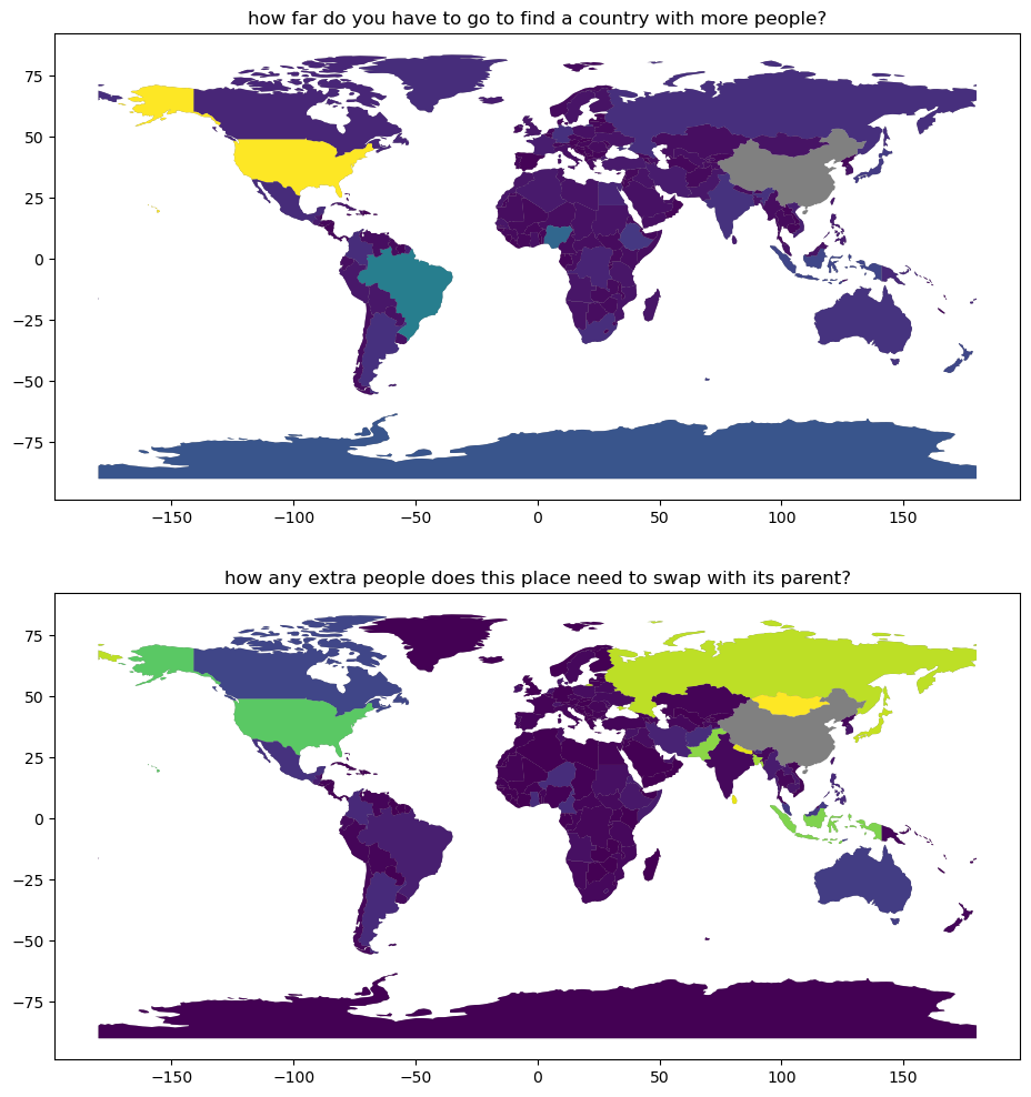
Visualizing this below, we get the following:

f, ax = plt.subplots(2, 1, figsize=(12, 12))
for i in range(2):
    natearth.plot(color="grey", ax=ax[i])
natearth.plot("isolation", ax=ax[0])
natearth.plot("gap", ax=ax[1])
ax[0].set_title("how far do you have to go to find a country with more people?")
ax[1].set_title("how any extra people does this place need to swap with its parent?")
plt.show()

Next, to see prominence, we’ll use the same arguments. However, prominence can also take a graph/libpysal.weights.W object that specifies the connections between sampled locations. If no pre-existing graph or surface is provided, the Delaunay Triangulation is used between the coordinates provided, which is a common triangulation in digital elevation models. Here, I’ll use the Rook contiguity graph, just for ease of interpretation. This means that some islands will automatically be considered as “peaks” because they don’t share any borders with any higher observations.

w_rook = weights.Rook.from_dataframe(natearth, use_index=False, silence_warnings=True)
prominence = topo.prominence(natearth["POP_EST"], w_rook, return_all=True)

Under the hood, this algorithm may take a bit longer for big data, so you can use the progressbar option to visualize the progress.

The actual algorithm entails sorting the data and determining whether we “connect” peaks together each time we introduce a new observation as equal to the declining sea level \(w\). We avoid re-computing scipy.sparse.connected_components each iteration by creating a set of neighbors for each “peak.” When two (or more) peaks merge, we replace the independent peaks i and j (where \(h_i > h_j\)) with peak (i,j). Each merge, the new peak gets the union of the sub-peaks neighbors, and are then treated as a single “peak” from then on.

We merge it back onto our data in the same fashion as before:

natearth = natearth.merge(
    prominence, left_index=True, right_index=True, suffixes=("", "_prom")
)

This gives us the following table. I’m going to show a bit more rows than usual so we can interpret it more clearly.

natearth[
    [
        "CONTINENT",
        "NAME",
        "POP_EST",
        "rank",
        "parent_rank",
        "isolation",
        "dominating_peak",
        "keycol",
        "prominence",
    ]
].sort_values("POP_EST", ascending=False).head(20)

	CONTINENT	NAME	POP_EST	rank	parent_rank	isolation	dominating_peak	keycol	prominence
139	Asia	China	1.397715e+09	0.0	NaN	NaN	139.0	107.0	1.314801e+09
98	Asia	India	1.366418e+09	1.0	0.0	27.852795	139.0	-1.0	NaN
4	North America	United States of America	3.282395e+08	2.0	1.0	193.538522	139.0	33.0	3.239931e+08
8	Asia	Indonesia	2.706256e+08	3.0	0.0	41.072699	4.0	148.0	2.386758e+08
102	Asia	Pakistan	2.165653e+08	4.0	1.0	12.381725	139.0	-1.0	NaN
29	South America	Brazil	2.110495e+08	5.0	2.0	82.093057	8.0	43.0	1.439896e+08
56	Africa	Nigeria	2.009636e+08	6.0	5.0	64.353456	29.0	55.0	1.776529e+08
99	Asia	Bangladesh	1.630462e+08	7.0	1.0	10.713323	139.0	-1.0	NaN
18	Europe	Russia	1.443735e+08	8.0	0.0	26.374718	139.0	-1.0	NaN
27	North America	Mexico	1.275755e+08	9.0	2.0	23.966775	4.0	-1.0	NaN
155	Asia	Japan	1.262649e+08	10.0	0.0	34.199305	56.0	-1.0	1.262648e+08
165	Africa	Ethiopia	1.120787e+08	11.0	6.0	31.568798	155.0	13.0	5.950476e+07
147	Asia	Philippines	1.081166e+08	12.0	3.0	15.020572	165.0	-1.0	1.081165e+08
163	Africa	Egypt	1.003881e+08	13.0	11.0	20.320874	147.0	14.0	5.757484e+07
94	Asia	Vietnam	9.646211e+07	14.0	12.0	17.322577	139.0	-1.0	NaN
11	Africa	Dem. Rep. Congo	8.679057e+07	15.0	11.0	19.680827	163.0	13.0	3.421659e+07
124	Asia	Turkey	8.342962e+07	16.0	13.0	13.623370	11.0	107.0	5.157090e+05
121	Europe	Germany	8.313280e+07	17.0	16.0	27.604762	124.0	43.0	1.607291e+07
107	Asia	Iran	8.291391e+07	18.0	4.0	15.341195	124.0	-1.0	0.000000e+00
91	Asia	Thailand	6.962558e+07	19.0	14.0	5.528840	121.0	93.0	1.558016e+07

These are the top 20 countries in terms of population. Walking down the rows, you see that China has a isolation of NaN and a prominence that is exactly equal to its population. India shares a border with China. So, when we “lower the sea level” to where India emerges from the water level, it’s already connected to the highest peak, China. So, its prominence is not very large. In fact, it’s considered a “slope” of the “China” mountain, and its dominating_peak is 139, the index for “China.” However, the US’s prominence is (confusingly) computed as the height relative to the population of Panama, sin ce Panama connects it to Sough America, where French Guyana then connects between NA/SA and Eurasia in this graph. Indonesia, likewise, has a prominence measured starting from Malaysia, which connects it to Asia, where it encounters the China-based subgraph.

For a visual on what the “key-cols” are, we’re thinking about the points at which the disconnected countries become connected in the following sequences of graphs. In each graph, only the “red” outlined countries are above the “water line” \(w\).

f, ax = plt.subplots(3, 2, figsize=(20, 20), sharex=True, sharey=True)
ax = ax.flatten()
for ix, rank in enumerate(range(5, 31, 5)):
    natearth.plot("classification", ax=ax[ix], cmap="Accent")
    natearth.sort_values("POP_EST", ascending=False).iloc[0:rank].boundary.plot(
        color="salmon", ax=ax[ix]
    )
    ax[ix].set_title(f"# of countries included: {rank}")
f.tight_layout()
plt.show()

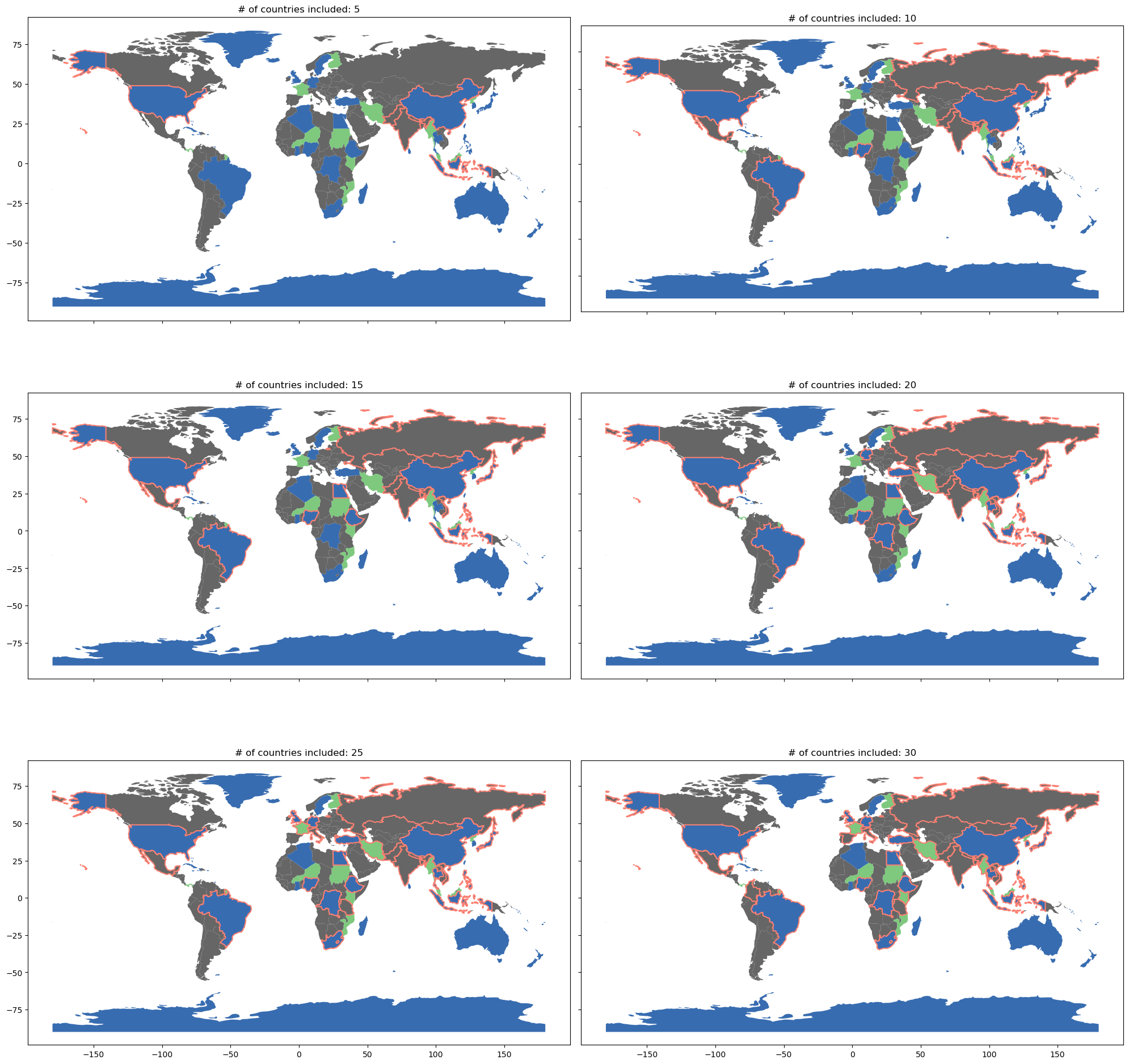
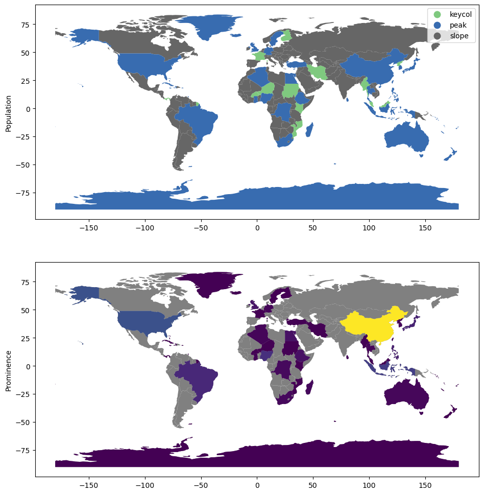
You can see that the first “key col” country, France, is included around the 25-country mark, wheras before that most included countries are “peaks,” disconnected from one another. Below, you can see the full map of classifications, alongside the prominence of each country.

f, ax = plt.subplots(2, 1, figsize=(12, 12))
natearth.plot("classification", ax=ax[0], legend=True, cmap="Accent")
natearth.plot(color="grey", ax=ax[1])
natearth.plot("prominence", ax=ax[1])
ax[0].set_ylabel("Population")
ax[1].set_ylabel("Prominence")
plt.show()