This page was generated from /home/runner/work/esda/esda/docs/notebooks/LOSH.ipynb. Interactive online version:

Assessing local patterns of spatial heteroskedasticity

In the following notebook we review the local spatial heteroskedasticity (LOSH) statistic (\(H_i\)) put forward by Ord and Getis (2012). LOSH is meant as an accompainment to the local statistics that analyze the mean level of a spatial process. LOSH focuses on analyzing the variance of the spatial process.

As outlined by Ord and Getis, consider a 10 x 10 grid of property values. Within this grid, there is a central high-rent district (identified by cells that are 1) and a surrounding lower-value area (identified by cells that are 0. We can visualize this spatial arrangement as:

0	0	0	0	0	0	0	0	0	0
0	0	0	0	0	0	0	0	0	0
0	0	0	0	0	0	0	0	0	0
0	0	0	1	1	1	1	0	0	0
0	0	0	1	1	1	1	0	0	0
0	0	0	1	1	1	1	0	0	0
0	0	0	1	1	1	1	0	0	0
0	0	0	0	0	0	0	0	0	0
0	0	0	0	0	0	0	0	0	0
0	0	0	0	0	0	0	0	0	0

While we can see that the inner core of the high-rent district have similar values to their neigbhors (i.e. a cells of 1 surrounded by other cells of 1), this is less true when we consider the outer rim of the high-rent district. This rim represents a possible transition region between the stable inner high-rent area and the stable outer lower value areas. Ord and Getis seek to use the LOSH statistic (\(H_i\)) to identify this transitional region between the two areas.

Understanding the LOSH statistic

Ord and Getis begin by defining a local mean, \(\bar{x}_i (d)\), as a re-scaled form of their \(G^*_i\) statistic. This local mean is:

Eq. 1

\[\bar{x}_i (d) = \frac{\sum_j w_{ij} (d) x_j}{\sum_j w_{ij}(d)}\]

With a local mean defined, we can understand local residuals as the value of a local unit minus the local mean, or:

Eq. 2

\[e_j(d) = x_j - \bar{x}_i(d), j \in N(i,d)\]

These local residuals may be incorporated into Eq. 1 to form a final local dispersion statistic called \(H_i\):

Eq. 3

\[H_i(d) = \frac{\sum w_{ij}(d) |e_j(d)|^a}{\sum w_{ij}(d)}\]

Note the addition of a new variable, \(a\). This handles the interpretation of the residuals. As explaiend by Ord and Getis:

When a = 1, we have an absolute deviations measure, Hi 1, and when a = 2 a variance measure, Hi2. Clearly, other choices are possible, along with various robust forms to avoid outliers. In order to produce a standard measure, we should divide by the mean absolute deviation or variance for the whole data set.

The default settings of the losh() function set \(a=2\).

Interpreting the LOSH statistic

Ord and Getis suggest that the \(H_i\) statistic may benefit from interpretation with the \(G^*_i\) statistic. The logic of this combined interpretation is that a the \(G^*_i\) value speaks to the local mean of the phenomenon of interest, whereas the \(H_i\) speaks to the local heterogeneity. Ord and Getis provide the following table as a simplified guide for interpretation:

Mean:nbsphinx-math:variance	High \(H_i\)	Low \(H_i\)
Large \(|G^*_i|\)	A hot spot with heterogeneous local conditions	A hot spot with similar surrounding areas; the map would indicate whether the affected region is larger than the single ‘cell’
Small \(|G^*_i|\)	Heterogeneous local conditions but at a low average level (an unlikely event)	Homogeneous local conditions and a low average level

Inference on the LOSH statistic

The current inference in the PySAL implementation of the LOSH statistic uses a \(\chi^2\) distribution. For each unit, we calculate a Z-score as:

\[Z_i = 2H_i / V_i\]

with \(2/V_i\) degrees of freedom. \(V_i\) is the local variance of the unit, calculated as:

\[Var_{p}(H_i) = \frac{1}{n-1} \left( \frac{1}{h_1 W_{i1}}\right) ^2 (h_2 - h_1^2) \left[nW_{i2} - W_{i1}^2\right]\]

It is worthwhile to note that alternative methods for inference have been proposed in Xu et al (2014). While these methods are not yet implemented in PySAL, they are available in the R spdep package as LOSH.mc. The PySAL function is comparable to the spdep LOSH and LOSH.cs functions.

Applying the LOSH statistic on a dataset

As a point of comparison, we now demonstrate the PySAL losh function on the Boston Housing Dataset, which is also used as the docexample in R spdep LOSH.cs. We are interested in the variable NOX, which is the ‘…vector of nitric oxides concentration (parts per 10 million) per town’.

We first load the Bostonhsg example dataset from libpysal:

import libpysal
import geopandas
boston = libpysal.examples.load_example('Bostonhsg')
boston_ds = geopandas.read_file(boston.get_path('boston.shp'))

/home/serge/anaconda3/envs/dev/lib/python3.8/site-packages/geopandas/_compat.py:84: UserWarning: The Shapely GEOS version (3.8.0-CAPI-1.13.1 ) is incompatible with the GEOS version PyGEOS was compiled with (3.8.1-CAPI-1.13.3). Conversions between both will be slow.
  warnings.warn(

Then we construct a Queen weight structure:

w = libpysal.weights.Queen.from_dataframe(boston_ds)

We can now import the losh() function. Note that it is in the form of a scikit-learn type estimator, so we pass both a series of arguments and then call .fit().

from esda.losh import LOSH
ls = LOSH(connectivity=w, inference="chi-square").fit(boston_ds['NOX'])

We can now examine the LOSH (\(H_i\)) values and their significance.

ls.Hi[0:10]

array([0.19690679, 0.51765774, 0.80382881, 0.80854441, 0.530667  ,
       0.525579  , 0.83291425, 0.84215733, 0.48875154, 0.41955327])

ls.pval[0:10]

array([0.86292242, 0.61157688, 0.45697742, 0.34426167, 0.57934554,
       0.55430556, 0.4135546 , 0.40999792, 0.54025022, 0.57801529])

If we want to map the LOSH (\(H_i\)) values, we need to add them back to the boston_ds dataframe.

boston_ds['Hi'] = ls.Hi
boston_ds['Hi_pval'] = ls.pval

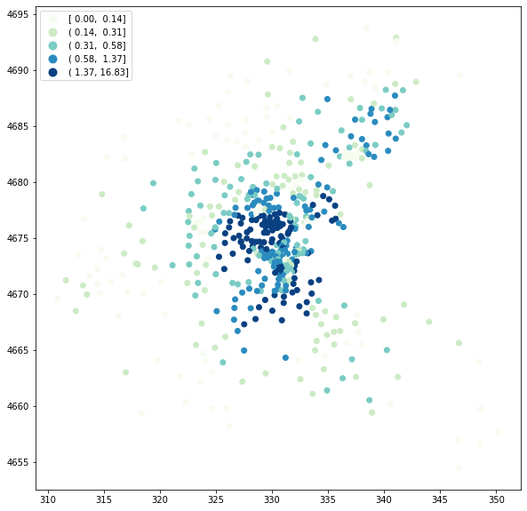
We can now map the LOSH (\(H_i\)) values. Note that we choose a Quantile break scheme here for visualization purposes.

import matplotlib.pyplot as plt
fig, ax = plt.subplots(figsize=(12,10), subplot_kw={'aspect':'equal'})
boston_ds.plot(column='Hi', scheme='Quantiles',
               k=5, cmap='GnBu',
               legend=True, ax=ax)

<AxesSubplot:>

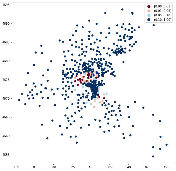
We can also examine significance of the values. We use cutoffs of 0.01, 0.05, 0.10, and above 0.10.

fig, ax = plt.subplots(figsize=(12,10), subplot_kw={'aspect':'equal'})
boston_ds.plot(column='Hi_pval', cmap='RdBu',
               legend=True, ax=ax,
               scheme='user_defined',
               classification_kwds={'bins':[0.01, 0.05, 0.10, 1]})

<AxesSubplot:>