This page was generated from notebooks/correlogram.ipynb. Interactive online version:

%load_ext watermark
%watermark -a 'eli knaap'
%load_ext autoreload
%autoreload 2

from libpysal import examples
from esda import correlogram

import geopandas as gpd

Author: eli knaap

sac = gpd.read_file(examples.load_example("Sacramento1").get_path("sacramentot2.shp"))

sac = sac.to_crs(sac.estimate_utm_crs())  # now in meters)

correlogram?

Signature:
correlogram(
    geometry: geopandas.geoseries.GeoSeries,
    variable: str | list | pandas.core.series.Series | None,
    support: list | None = None,
    statistic: collections.abc.Callable | str = <class 'esda.moran.Moran'>,
    distance_type: str = 'band',
    weights_kwargs: dict = None,
    stat_kwargs: dict = None,
    select_numeric: bool = False,
    n_jobs: int = -1,
    n_bins: int | None = 50,
) -> pandas.core.frame.DataFrame
Docstring:
Generate a spatial correlogram

A spatial profile is a set of spatial autocorrelation statistics calculated for
a set of increasing distances. It is a useful exploratory tool for examining
how the relationship between spatial units changes over different notions of scale.

Parameters
----------
geometry : gpd.GeoSeries
    geodataframe holding spatial and attribute data
variable: pd.Series or list
    pandas series matching input geometries
support : list or None
    list of values at which to compute the autocorrelation statistic
statistic : callable or str
    statistic to be computed for a range of libpysal.Graph specifications.
    This should be a class with a signature like `Statistic(y,w, **kwargs)`
    where y is a  array and w is a libpysal.weights.W object
    Generally, this is a class from pysal's `esda` package
    defaults to esda.Moran, which computes the Moran's I statistic. If
    'lowess' is provided, a non-parametric correlogram is computed using
    lowess regression on the spatial-covariation model, see Notes.
distance_type : str, optional
    which concept of distance to increment. Options are {`band`, `knn`}.
    by default 'band' (for `libpysal.weights.DistanceBand` weights)
weights_kwargs : dict
    additional keyword arguments passed to the libpysal.weights.W class
stat_kwargs : dict
    additional keyword arguments passed to the `esda` autocorrelation statistic class.
    For example for faster results with no statistical inference, set the number
    of permutations to zero with stat_kwargs={permutations: 0}
select_numeric : bool
    if True, only return numeric attributes from the original class. This is useful
    e.g. to prevent lists inside a "cell" of a dataframe
n_jobs : int
    number of jobs to pass to joblib. If -1 (default), all cores will be used
n_bins : int
    number of distance bands or k-nearest neighbor values to use if
    `support` is not provided. Ignored if `support` is provided.
    by default 10. If `distance_type` is 'knn', the number of neighbors
    will be capped at n-1, where n is the number of observations. Further,
    if n-1 is not divisible by `n_bins`, the actual number of bins will be
    may be off by one bin.

Returns
-------
outputs : pandas.DataFrame
    table of autocorrelation statistics at increasing distance bandwidths

Notes
-----
The nonparametric correlogram uses a lowess regression
to estimate the spatial-covariation model:

    zi*zj = f(d_{ij}) + e_ij

where f is a smooth function of distance d_{ij} between points i and j.
This function requires the statsmodels package to be installed.

For the nonparametric correlogram, a precomputed distance matrix can
be used. To do this, set
stat_kwargs={'metric':'precomputed', 'coordinates':distance_matrix}
where `distance_matrix` is a square matrix of pairwise distances that
aligns with the `geometry` rows.
File:      ~/Dropbox/work/dev/esda/esda/correlogram.py
Type:      function

from esda import Moran, Geary, G

Distance Bands

# Create a liste of distances between 500 and 5000 (meters, here) in increments of 500

distances = [i+500 for i in range(0,5000, 500)]

distances

[500, 1000, 1500, 2000, 2500, 3000, 3500, 4000, 4500, 5000]

The correlogram will compute an autocorrelation statistic (Moran’s \(I\) by default) at each distance threshold. Plotting this statistic against distance reveals how spatial similarity changes over distance (similar in concept to a variogram)

prof = correlogram(
    sac.centroid,
    sac.HH_INC,
    distances,
    Moran
)

prof is a dataframe of autocorrelation statistics indexed by distance. It includes all attributes created by the esda autocorrelation statistic class (e.g. Moran, Geary, or Geits-Ord G). The row index for each statistic is the distance at which it was computed

prof.head()

	y	w	permutations	n	z	z2ss	EI	VI_norm	seI_norm	VI_rand	...	z_rand	p_norm	p_rand	sim	p_sim	EI_sim	seI_sim	VI_sim	z_sim	p_z_sim
500	[52941, 51958, 32992, 54556, 50815, 60167, 490...	<libpysal.weights.distance.DistanceBand object...	999	403	[0.27506115837390277, 0.21948138443207246, -0....	1.260604e+11	-0.002488	0.497534	0.705361	0.496239	...	0.086188	9.314058e-01	9.313166e-01	[-0.041149125017795225, 0.8047828919464444, 0....	0.465	-0.017506	0.693436	0.480854	0.109214	4.565164e-01
1000	[52941, 51958, 32992, 54556, 50815, 60167, 490...	<libpysal.weights.distance.DistanceBand object...	999	403	[0.27506115837390277, 0.21948138443207246, -0....	1.260604e+11	-0.002488	0.014259	0.119409	0.014221	...	4.147088	3.447621e-05	3.367309e-05	[0.01407910066509541, -0.09399265148441757, -0...	0.001	-0.007273	0.120349	0.014484	4.149132	1.668694e-05
1500	[52941, 51958, 32992, 54556, 50815, 60167, 490...	<libpysal.weights.distance.DistanceBand object...	999	403	[0.27506115837390277, 0.21948138443207246, -0....	1.260604e+11	-0.002488	0.004586	0.067719	0.004574	...	6.763620	1.430242e-11	1.345857e-11	[-0.028776580865062164, 0.07946937157388524, 0...	0.001	-0.003352	0.067581	0.004567	6.781418	5.950106e-12
2000	[52941, 51958, 32992, 54556, 50815, 60167, 490...	<libpysal.weights.distance.DistanceBand object...	999	403	[0.27506115837390277, 0.21948138443207246, -0....	1.260604e+11	-0.002488	0.002164	0.046515	0.002158	...	12.164298	5.846476e-34	4.815656e-34	[-0.0566559868640034, 0.06456200403436937, -0....	0.001	-0.000508	0.047756	0.002281	11.791263	2.164994e-32
2500	[52941, 51958, 32992, 54556, 50815, 60167, 490...	<libpysal.weights.distance.DistanceBand object...	999	403	[0.27506115837390277, 0.21948138443207246, -0....	1.260604e+11	-0.002488	0.001481	0.038483	0.001477	...	13.102771	3.974924e-39	3.174519e-39	[-0.03272028047068946, -0.025327634962963246, ...	0.001	-0.002785	0.039315	0.001546	12.816543	6.623787e-38

5 rows × 23 columns

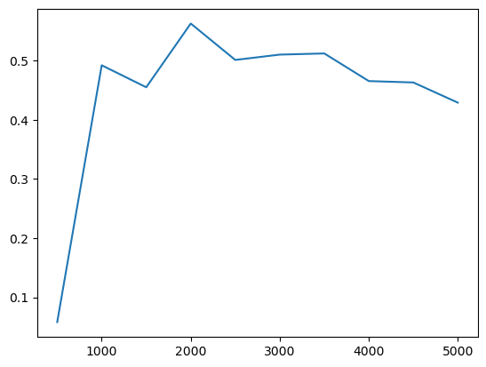
Often, it is easiest to visualize the statistic, and the pandas plot function will plot a column against the dataframe’s index by default

ax = prof.I.plot()
ax.set_xlabel("distance (m)")
ax.set_ylabel("Moran's I")

<Axes: >

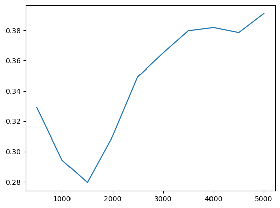
Autocorrelation statistics differ in concept, so the shape of the spatial correlogram statistic will vary considerably, based on which statistic is created. For example, we can also plot Geary’s \(C\)

prof = correlogram(
    sac.centroid,
    sac.HH_INC,
    distances,
    statistic=Geary
)

ax = prof.C.plot()
ax.set_xlabel("distance (m)")
ax.set_ylabel("Geary's C")

<Axes: >

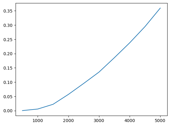
…Or Getis-Ord \(G\)

prof = correlogram(
    sac.centroid,
    sac.HH_INC,
    distances,
    statistic=G
)

ax = prof.G.plot()
ax.set_xlabel("distance (m)")
ax.set_ylabel("Getis-Ord G")

<Axes: >

You can also leave the distance thresholds unspecified, and the correlogram will estimate over a reasonable range of distances:

prof = correlogram(
    sac.centroid,
    sac.HH_INC,
    statistic=G
)
ax = prof.G.plot()
ax.set_xlabel("distance (m)")
ax.set_ylabel("Getis-Ord G")

<Axes: >

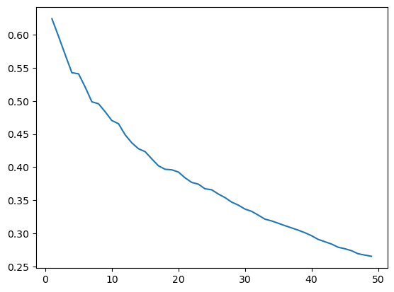
KNN Distance

It is also possible to consider different concepts of distance. For example, rather than stepping through increments of Euclidean distance/length at each interval, we could instead step through increments of nearest-neighbors.

Instead of adding neighbors using sequential distances of 500 meters, here we will step through the 50 nearest neighbors, adding one neighbor at a time

kdists = list(range(1,50))

kcorr = correlogram(sac.centroid, sac.HH_INC, kdists, distance_type='knn')

ax = kcorr.I.plot()
ax.set_xlabel("number of nearest neighbors")
ax.set_ylabel("Moran's I")

<Axes: >

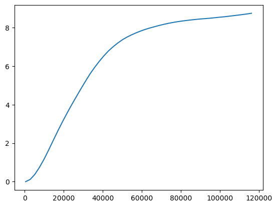
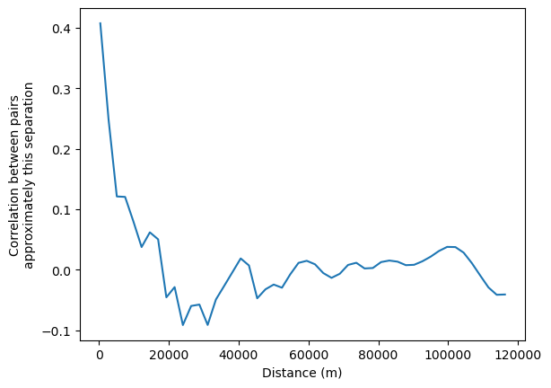
Nonparametric

Finally it is also possible to fit a non-parametric curve to estimate spatial autocorrelation as a function of distance. This is done using a LOWESS smoother, which fits a locally-weighted polynomial regression to the data based on the following regression:

\[z_iz_j = f(d_{ij}) + u_{ij}\]

where \(z_i\) and \(z_j\) are standardized values of the variable of interest at locations \(i\) and \(j\), \(d_{ij}\) is the distance between locations \(i\) and \(j\), and \(u_{ij}\) is an error term. The function \(f\) is estimated using a LOWESS smoother, which fits a locally-weighted polynomial regression to the data.

This can be interpreted as the correlation between observations separated by approximately the distance on the horizontal axis.

nonparametric = correlogram(sac.centroid, sac.HH_INC, statistic='lowess')
ax = nonparametric.lowess.plot()
ax.set_xlabel("Distance (m)")
ax.set_ylabel("Correlation between pairs\napproximately this separation")

Text(0, 0.5, 'Correlation between pairs\napproximately this separation')