Ensemble models
gwlearn implements geographically weighted versions of ensemble models for both classification and regression tasks. For classification, there’s a caveat: given it is unlikely that all categories are present in all local models, fitting a non-binary would lead to inconsistent local models. Hence gwlearn currently supports only binary classification.
This notebook outlines how to fit the models and extract their attributes. For details on prediction, see the Prediction guide.
import geopandas as gpd
from geodatasets import get_path
from sklearn import metrics

from gwlearn.ensemble import (
    GWGradientBoostingClassifier,
    GWGradientBoostingRegressor,
    GWRandomForestClassifier,
    GWRandomForestRegressor,
)
Get sample data
gdf = gpd.read_file(get_path("geoda.south")).to_crs(5070)

gdf["point"] = gdf.representative_point()
gdf = gdf.set_geometry("point")

y = gdf["FH90"] > gdf["FH90"].median()  # binary target for classification
X = gdf.iloc[:, 9:15]
Random Forest Classifier
The implementation of geographically-weighted random forest classifier follows the logic of linear models, where each local neighborhood defined by a set bandwidth is used to fit a single local model.
gwrf = GWRandomForestClassifier(
    bandwidth=150,
    fixed=False,
)
gwrf.fit(
    X,
    y,
    geometry=gdf.geometry,
)
GWRandomForestClassifier(bandwidth=150)In a Jupyter environment, please rerun this cell to show the HTML representation or trust the notebook.
On GitHub, the HTML representation is unable to render, please try loading this page with nbviewer.org.
Parameters
| bandwidth | 150 | |
| fixed | False | |
| kernel | 'bisquare' | |
| include_focal | False | |
| graph | None | |
| n_jobs | -1 | |
| fit_global_model | True | |
| strict | False | |
| keep_models | False | |
| temp_folder | None | |
| batch_size | None | |
| min_proportion | 0.2 | |
| undersample | False | |
| leave_out | None | |
| random_state | None | |
| verbose | False |
Focal score
The performance of these models can be measured in three ways. The first one is using the focal prediction. Unlike in linear models, where the focal observation is part of the local model training, in this case it is excluded to ensure it can be used to evaluate the model. Otherwise, it would be a part of the data the local model has seen and would report unrealistically high performance. If you want to include the focal observation in the training nevertheless, just set include_focal=True.
Focal accuracy can be measured as follows. Note that some local models are not fitted due to imbalance rules, and report NA that needs to be filtered out.
na_mask = gwrf.pred_.notna()

metrics.accuracy_score(y[na_mask], gwrf.pred_[na_mask])
0.7595258255715496
Pooled out-of-bag score
Another option is to pull the out-of-bag predictions from individual local models and pool them together. This uses more data to evaluate the model but given the local models are tuned for their focal location, some predictions on locations far from the focal point may be artifically worse than the actual model prediction would be.
metrics.accuracy_score(gwrf.oob_y_pooled_, gwrf.oob_pred_pooled_)
0.7442901495907424
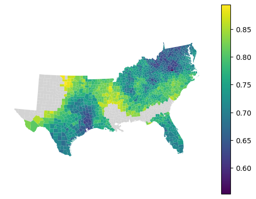
Local score
The final option is to take the local out-of-bag predicitons and measure performance per each local model. To do that, you can use a method local_metric().
local_accuracy = gwrf.local_metric(metrics.accuracy_score)
local_accuracy
array([0.66666667, 0.68666667, 0.72      , ..., 0.62      , 0.72      ,
       0.68666667], shape=(1412,))
gdf.set_geometry("geometry").plot(
    local_accuracy, legend=True, missing_kwds=dict(color="lightgray")
).set_axis_off()
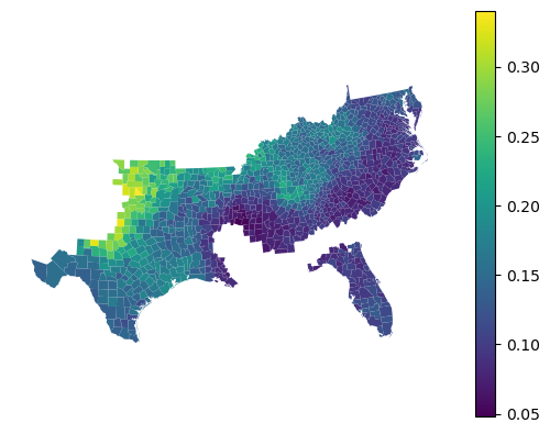
Feature importance
Feature importances are reported for each local model.
gwrf.feature_importances_
| HR60 | HR70 | HR80 | HR90 | HC60 | HC70 | |
|---|---|---|---|---|---|---|
| 0 | 0.179199 | 0.183928 | 0.190695 | 0.213653 | 0.107877 | 0.124649 |
| 1 | 0.181576 | 0.169348 | 0.183969 | 0.220722 | 0.107891 | 0.136494 |
| 2 | 0.174052 | 0.176314 | 0.188204 | 0.241107 | 0.127007 | 0.093315 |
| 3 | 0.174124 | 0.173054 | 0.187784 | 0.240875 | 0.120061 | 0.104102 |
| 4 | 0.135409 | 0.156295 | 0.221974 | 0.221731 | 0.116691 | 0.147900 |
| ... | ... | ... | ... | ... | ... | ... |
| 1407 | 0.132448 | 0.178123 | 0.267094 | 0.243993 | 0.080124 | 0.098217 |
| 1408 | 0.182823 | 0.163517 | 0.212140 | 0.233453 | 0.106007 | 0.102060 |
| 1409 | 0.140616 | 0.180056 | 0.209712 | 0.213265 | 0.134399 | 0.121952 |
| 1410 | 0.153820 | 0.208140 | 0.224005 | 0.168249 | 0.108178 | 0.137610 |
| 1411 | 0.147265 | 0.183170 | 0.233029 | 0.199166 | 0.115051 | 0.122320 |
1412 rows × 6 columns
gdf.set_geometry("geometry").plot(
    gwrf.feature_importances_["HC60"], legend=True
).set_axis_off()
You can compare all of this to values extracted from a global model, fitted alongside.
gwrf.global_model.feature_importances_
array([0.14155788, 0.15740365, 0.22588841, 0.25075606, 0.10676568,
       0.11762833])
gwrf.feature_importances_.mean()
HR60    0.154666
HR70    0.159607
HR80    0.202272
HR90    0.221558
HC60    0.139777
HC70    0.122120
dtype: float64
Random Forest Regressor
The GWRandomForestRegressor provides the same functionality as the classifier version but for continuous target variables. It uses local Random Forest models to capture spatial heterogeneity in regression relationships.
y_reg = gdf["FH90"]
gwrf_reg = GWRandomForestRegressor(
    bandwidth=150,
    fixed=False,
    random_state=0,
)
gwrf_reg.fit(
    X,
    y_reg,
    geometry=gdf.representative_point(),
)
GWRandomForestRegressor(bandwidth=150, random_state=0)In a Jupyter environment, please rerun this cell to show the HTML representation or trust the notebook.
On GitHub, the HTML representation is unable to render, please try loading this page with nbviewer.org.
Parameters
| bandwidth | 150 | |
| fixed | False | |
| kernel | 'bisquare' | |
| include_focal | False | |
| graph | None | |
| n_jobs | -1 | |
| fit_global_model | True | |
| strict | False | |
| keep_models | False | |
| temp_folder | None | |
| batch_size | None | |
| random_state | 0 | |
| verbose | False |
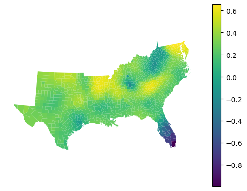
The regressor provides local R² values showing how well the model fits in each neighborhood:
gwrf_reg.local_r2_.head()
0    0.104145
1    0.035537
2   -0.039846
3   -0.048805
4    0.637768
dtype: float64
gdf.set_geometry("geometry").plot(gwrf_reg.local_r2_, legend=True).set_axis_off()
Out-of-bag performance
Like the classifier, the regressor supports out-of-bag predictions that can be used to evaluate model performance:
from sklearn.metrics import r2_score

r2_score(gwrf_reg.oob_y_pooled_, gwrf_reg.oob_pred_pooled_)
0.5014741368618677
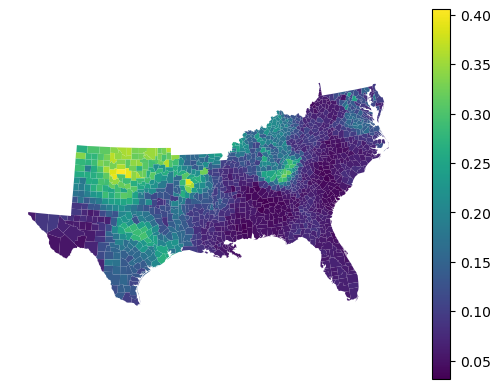
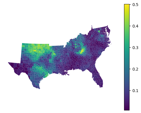
Feature importance
Feature importances show the contribution of each feature in local models:
gwrf_reg.feature_importances_.head()
| HR60 | HR70 | HR80 | HR90 | HC60 | HC70 | |
|---|---|---|---|---|---|---|
| 0 | 0.112869 | 0.177485 | 0.180982 | 0.265641 | 0.073176 | 0.189846 |
| 1 | 0.114309 | 0.146802 | 0.172446 | 0.288038 | 0.075410 | 0.202995 |
| 2 | 0.152714 | 0.153546 | 0.180235 | 0.331140 | 0.057873 | 0.124492 |
| 3 | 0.140662 | 0.157790 | 0.169440 | 0.305476 | 0.051538 | 0.175094 |
| 4 | 0.048769 | 0.071535 | 0.307233 | 0.300384 | 0.095678 | 0.176401 |
gdf.set_geometry("geometry").plot(
    gwrf_reg.feature_importances_["HC60"], legend=True
).set_axis_off()
Gradient Boosting Classifier
If you prefer to use gradient boosting, there is a minimal implementation of geographically weighted gradient boosting classifier, following the same model described for the random forest above.
gwgb = GWGradientBoostingClassifier(
    bandwidth=150,
    fixed=False,
)
gwgb.fit(
    X,
    y,
    geometry=gdf.geometry,
)
GWGradientBoostingClassifier(bandwidth=150)In a Jupyter environment, please rerun this cell to show the HTML representation or trust the notebook.
On GitHub, the HTML representation is unable to render, please try loading this page with nbviewer.org.
Parameters
| bandwidth | 150 | |
| fixed | False | |
| kernel | 'bisquare' | |
| include_focal | False | |
| graph | None | |
| n_jobs | -1 | |
| fit_global_model | True | |
| strict | False | |
| keep_models | False | |
| temp_folder | None | |
| batch_size | None | |
| min_proportion | 0.2 | |
| undersample | False | |
| random_state | None | |
| verbose | False |
Given the nature of the model, the outputs are a bit more limited. You can still extract focal predictions.
nan_mask = gwgb.pred_.notna()

metrics.accuracy_score(y[nan_mask], gwgb.pred_[nan_mask])
0.7502116850127011
And local feature importances.
gwgb.feature_importances_
| HR60 | HR70 | HR80 | HR90 | HC60 | HC70 | |
|---|---|---|---|---|---|---|
| 0 | 0.158903 | 0.259769 | 0.186528 | 0.223505 | 0.078761 | 0.092534 |
| 1 | 0.191966 | 0.173055 | 0.209454 | 0.232258 | 0.073896 | 0.119371 |
| 2 | 0.234714 | 0.123025 | 0.179186 | 0.290409 | 0.062696 | 0.109970 |
| 3 | 0.161227 | 0.210035 | 0.169236 | 0.267748 | 0.105018 | 0.086737 |
| 4 | 0.071988 | 0.179369 | 0.253934 | 0.242457 | 0.093461 | 0.158791 |
| ... | ... | ... | ... | ... | ... | ... |
| 1407 | 0.120854 | 0.171583 | 0.382890 | 0.256796 | 0.031084 | 0.036794 |
| 1408 | 0.229032 | 0.139042 | 0.284922 | 0.209077 | 0.093431 | 0.044496 |
| 1409 | 0.125254 | 0.288581 | 0.248684 | 0.207918 | 0.088088 | 0.041475 |
| 1410 | 0.123648 | 0.229589 | 0.263491 | 0.229434 | 0.031265 | 0.122573 |
| 1411 | 0.069533 | 0.186643 | 0.330154 | 0.243639 | 0.114186 | 0.055845 |
1412 rows × 6 columns
Leave out samples
However, the pooled data are not available. In this case, you can use the leave_out keyword to leave out a fraction (when float) or a set number (when int) of random observations from each local model. For these, the local model does prediction and returns as left_out_proba_ and left_out_y_ arrays.
gwgb_leave = GWGradientBoostingClassifier(
    bandwidth=150,
    fixed=False,
    leave_out=0.2,
)
gwgb_leave.fit(
    X,
    y,
    geometry=gdf.geometry,
)
GWGradientBoostingClassifier(bandwidth=150)In a Jupyter environment, please rerun this cell to show the HTML representation or trust the notebook.
On GitHub, the HTML representation is unable to render, please try loading this page with nbviewer.org.
Parameters
| bandwidth | 150 | |
| fixed | False | |
| kernel | 'bisquare' | |
| include_focal | False | |
| graph | None | |
| n_jobs | -1 | |
| fit_global_model | True | |
| strict | False | |
| keep_models | False | |
| temp_folder | None | |
| batch_size | None | |
| min_proportion | 0.2 | |
| undersample | False | |
| random_state | None | |
| verbose | False |
metrics.accuracy_score(
    gwgb_leave.left_out_y_, gwgb_leave.left_out_proba_.argmax(axis=1)
)
0.7224103866779565
Gradient Boosting Regressor
In the GWGradientBoostingRegressor, gradient boosting is applied for regression, taking into consideration the spatial heterogeneity. Gradient boosting is a type of boosting that builds a model by adding trees on a sequentially iterative basis; every new tree attempts to predict the errors made by the preceding ensemble. This makes the gradient boosting regressor appropriately suited for modeling complex non-linear relationships.
Unlike Random Forest, out-of-bag predictions are not implemented for Gradient Boosting in gwlearn. If you want to evaluate your model without a separate test dataset, you can use the leave_out option (as shown in the classifier section) or consider using GWRandomForestRegressor, which provides built-in OOB scoring.
gwgb_reg = GWGradientBoostingRegressor(
    bandwidth=150,
    fixed=False,
    random_state=0,
)
gwgb_reg.fit(
    X,
    y_reg,
    geometry=gdf.representative_point(),
)
GWGradientBoostingRegressor(bandwidth=150, random_state=0)In a Jupyter environment, please rerun this cell to show the HTML representation or trust the notebook.
On GitHub, the HTML representation is unable to render, please try loading this page with nbviewer.org.
Parameters
| bandwidth | 150 | |
| fixed | False | |
| kernel | 'bisquare' | |
| include_focal | False | |
| graph | None | |
| n_jobs | -1 | |
| fit_global_model | True | |
| strict | False | |
| keep_models | False | |
| temp_folder | None | |
| batch_size | None | |
| random_state | 0 | |
| verbose | False |
The regressor provides local R² values showing how well the model fits in each neighborhood:
gwgb_reg.local_r2_.head()
0   -0.063802
1   -0.160997
2   -0.276301
3   -0.262151
4    0.596555
dtype: float64
gdf.set_geometry('geometry').plot(gwgb_reg.local_r2_, legend=True).set_axis_off()
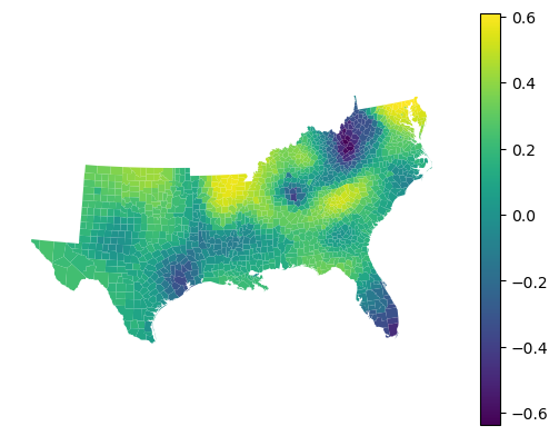
Feature importance
Gradient boosting computes feature importances based on how much each feature reduces the loss function across all trees in the ensemble. These importances tend to be more focused on the most predictive features compared to Random Forest:
gwgb_reg.feature_importances_.head()
| HR60 | HR70 | HR80 | HR90 | HC60 | HC70 | |
|---|---|---|---|---|---|---|
| 0 | 0.085339 | 0.135627 | 0.223552 | 0.292395 | 0.066986 | 0.196100 |
| 1 | 0.099639 | 0.131126 | 0.157998 | 0.319981 | 0.049697 | 0.241560 |
| 2 | 0.085873 | 0.142108 | 0.213703 | 0.413821 | 0.033547 | 0.110948 |
| 3 | 0.100750 | 0.146411 | 0.176120 | 0.374961 | 0.024218 | 0.177541 |
| 4 | 0.028554 | 0.049572 | 0.344836 | 0.462574 | 0.030520 | 0.083944 |
gdf.set_geometry('geometry').plot(gwgb_reg.feature_importances_["HC60"], legend=True).set_axis_off()
Comparison with global model
You can compare the local feature importances to values from the global model:
gwgb_reg.global_model.feature_importances_
array([0.06612286, 0.10260245, 0.20458955, 0.45924727, 0.10816795,
       0.05926993])
gwgb_reg.feature_importances_.mean()
HR60    0.127108
HR70    0.121543
HR80    0.222230
HR90    0.302311
HC60    0.123322
HC70    0.103485
dtype: float64