Bandwidth search
To find out the optimal bandwidth, gwlearn provides a BandwidthSearch class, which trains models on a range of bandwidths and selects the most optimal one.
import geopandas as gpd
from geodatasets import get_path

from gwlearn.linear_model import GWLinearRegression, GWLogisticRegression
from gwlearn.search import BandwidthSearch
Get sample data
gdf = gpd.read_file(get_path("geoda.south")).to_crs(5070)

gdf["point"] = gdf.representative_point()
gdf = gdf.set_geometry("point")

y = gdf["FH90"]
X = gdf.iloc[:, 9:15]
Downloading file 'south.zip' from 'https://geodacenter.github.io/data-and-lab//data/south.zip' to '/home/runner/.cache/geodatasets'.
Extracting 'south/south.gpkg' from '/home/runner/.cache/geodatasets/south.zip' to '/home/runner/.cache/geodatasets/south.zip.unzip'
Interval search
Interval search tests the model at a set interval.
search = BandwidthSearch(
    GWLinearRegression,
    fixed=False,
    n_jobs=-1,
    search_method="interval",
    min_bandwidth=50,
    max_bandwidth=1000,
    interval=100,
    criterion="aicc",
    verbose=True,
)
search.fit(
    X,
    y,
    geometry=gdf.geometry,
)
Bandwidth: 50.00, aicc: 7685.453
Bandwidth: 150.00, aicc: 7598.040
Bandwidth: 250.00, aicc: 7672.563
Bandwidth: 350.00, aicc: 7722.884
Bandwidth: 450.00, aicc: 7764.566
Bandwidth: 550.00, aicc: 7811.208
Bandwidth: 650.00, aicc: 7862.718
Bandwidth: 750.00, aicc: 7904.325
Bandwidth: 850.00, aicc: 7941.803
Bandwidth: 950.00, aicc: 7981.327
<gwlearn.search.BandwidthSearch at 0x7fcb20ed23c0>
The scores_ series then contains the AICc, selected as the criterion, which can be plotted to see the change of the model performance as the bandwidth grows.
search.scores_.plot()
<Axes: >
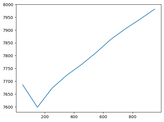
The optimal bandwidth is then the lowest one.
search.optimal_bandwidth_
np.int64(150)
Golden section
Alternatively, you can try to use the golden section algorithm that attempts to find the optimal bandwidth iteratively. However, note that there’s no guaratnee that it will find the globally optimal bandwidth as it may stick to the local minimum.
search = BandwidthSearch(
    GWLinearRegression,
    fixed=True,
    n_jobs=-1,
    search_method="golden_section",
    criterion="aicc",
    min_bandwidth=10_000,
    max_bandwidth=1_000_000,
    verbose=True,
)
search.fit(
    X,
    y,
    geometry=gdf.geometry,
)
Bandwidth: 388150.3, score: 7669.800
Bandwidth: 621849.7, score: 7770.467
Bandwidth: 243708.23, score: 7595.916
Bandwidth: 154442.07, score: 7909.632
Bandwidth: 298880.77, score: 7625.628
Bandwidth: 209613.32, score: 7615.954
Bandwidth: 264783.28, score: 7604.069
Bandwidth: 230686.59, score: 7596.427
Bandwidth: 251759.37, score: 7598.529
Bandwidth: 238735.76, score: 7595.231
Bandwidth: 235660.47, score: 7595.389
Bandwidth: 240634.23, score: 7595.329
Bandwidth: 237560.29, score: 7595.268
Bandwidth: 239460.08, score: 7595.241
<gwlearn.search.BandwidthSearch at 0x7fcac06f5d10>
You can see how the agorithm searches and iteratively gets closer to the optimum.
search.optimal_bandwidth_
np.float64(238735.7582789531)
Other metrics
By default, BandwidthSearch computes AICc, AIC and BIC, available through metrics_.
search.metrics_
| aicc | aic | bic | |
|---|---|---|---|
| 388150.300000 | 7669.800284 | 7650.730706 | 8238.208833 |
| 621849.700000 | 7770.467076 | 7766.321405 | 8047.693794 |
| 243708.229909 | 7595.915658 | 7497.313206 | 8762.156146 |
| 154442.070091 | 7909.631563 | 7355.237895 | 9995.188728 |
| 298880.767422 | 7625.628201 | 7578.766844 | 8477.096909 |
| 209613.319310 | 7615.953544 | 7443.545102 | 9065.985674 |
| 264783.280267 | 7604.069091 | 7531.986411 | 8628.488146 |
| 230686.589297 | 7596.426806 | 7475.433826 | 8862.323769 |
| 251759.367217 | 7598.528817 | 7511.192286 | 8708.266105 |
| 238735.758279 | 7595.231162 | 7488.668425 | 8798.649792 |
| 235660.465361 | 7595.389267 | 7483.564238 | 8822.281852 |
| 240634.225285 | 7595.328622 | 7491.905192 | 8784.335011 |
| 237560.292439 | 7595.268103 | 7486.713835 | 8807.668987 |
| 239460.075156 | 7595.240977 | 7489.889063 | 8793.138119 |
You can also ask for a log loss and even use it as a criterion for the selection. This is useful when comparing classification models with varying prediction rate (you can also retrieve that for each bandwidth).
search = BandwidthSearch(
    GWLogisticRegression,
    fixed=False,
    n_jobs=-1,
    search_method="interval",
    min_bandwidth=50,
    max_bandwidth=1000,
    interval=200,
    metrics=["log_loss", "prediction_rate"],
    criterion="log_loss",
    verbose=True,
)
search.fit(
    X,
    y > y.median(),  # simulate binary categorical variable
    geometry=gdf.geometry,
)
Bandwidth: 50.00, log_loss: 0.276
Bandwidth: 250.00, log_loss: 0.376
Bandwidth: 450.00, log_loss: 0.413
Bandwidth: 650.00, log_loss: 0.437
Bandwidth: 850.00, log_loss: 0.454
<gwlearn.search.BandwidthSearch at 0x7fcac8224f50>
Log loss is then part of the metrics.
search.metrics_
| aicc | aic | bic | log_loss | prediction_rate | |
|---|---|---|---|---|---|
| 50 | 1376.806547 | 1119.216534 | 2551.160957 | 0.275782 | 0.682011 |
| 250 | 1262.969346 | 1249.800971 | 1741.819969 | 0.376227 | 1.000000 |
| 450 | 1275.319005 | 1271.315792 | 1547.948404 | 0.412885 | 1.000000 |
| 650 | 1308.172651 | 1306.304157 | 1497.258268 | 0.436826 | 1.000000 |
| 850 | 1337.777857 | 1336.720382 | 1481.487638 | 0.453824 | 1.000000 |
And is reported directly as score as it is set as the criterion.
search.scores_.plot()
<Axes: >
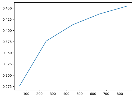
As a result, the optimal bandwidth is derived directly from it.
search.optimal_bandwidth_
np.int64(50)