Class imbalance
Class imbalance across the space can be a serious issue when trying to build a geographically weighted classification model. You can get to such extreme situations, that all of the observations within the set bandwidth share a single value. In that case, fitting a model that would predicting anything else than that value is not possible.
Even in less extreme cases, the class imbalance can induce bias to the local model.
import geopandas as gpd
import numpy as np
from geodatasets import get_path
from sklearn import metrics

from gwlearn.ensemble import GWRandomForestClassifier
Initial situation
Use the Guerry dataset and create a binary variable to predict. Use a subset of other columns as explanatory variables.
gdf = gpd.read_file(get_path("geoda.guerry"))
y = gdf["Suicids"] > gdf["Suicids"].median()
X = gdf[['Crm_prp', 'Litercy', 'Donatns', 'Lottery']]
Fit the model using the default settings.
model = GWRandomForestClassifier(
    geometry=gdf.representative_point(),
    bandwidth=25,
    fixed=False,
)
model.fit(
    X,
    y,
)
GWRandomForestClassifier(bandwidth=25,
                         geometry=0     POINT (827911.875 2122906.5)
1       POINT (691725.716 2496059)
2     POINT (663520.408 2152677.5)
3       POINT (908864.897 1915755)
4     POINT (916568.259 1968489.5)
                  ...
80      POINT (322806.903 2192566)
81      POINT (456440.882 2181291)
82     POINT (510125.65 2102842.5)
83      POINT (901963.264 2362015)
84       POINT (697522.96 2318253)
Length: 85, dtype: geometry)
In a Jupyter environment, please rerun this cell to show the HTML representation or trust the notebook. On GitHub, the HTML representation is unable to render, please try loading this page with nbviewer.org.
Parameters
| bandwidth | 25 | |
| fixed | False | |
| kernel | 'bisquare' | |
| include_focal | False | |
| geometry | 0 POINT (...type: geometry | |
| graph | None | |
| n_jobs | -1 | |
| fit_global_model | True | |
| strict | False | |
| keep_models | False | |
| temp_folder | None | |
| batch_size | None | |
| min_proportion | 0.2 | |
| undersample | False | |
| leave_out | None | |
| random_state | None | |
| verbose | False |
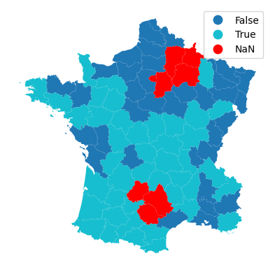
By default, the class imbalance affects which models are fitted and which are not. The default for the min_proportion parameter is 0.2, meaning the minority class needs to occur in at least 20% of observations within a local bandwidth. Otherwise, the model is not fitted. You can check how many local models are fitted under these conditions.
model.prediction_rate_
np.float64(0.9058823529411765)
You can see that visually if you map the outcome of the focal prediction.
gdf.plot(model.pred_, missing_kwds=dict(color='red'), legend=True).set_axis_off()
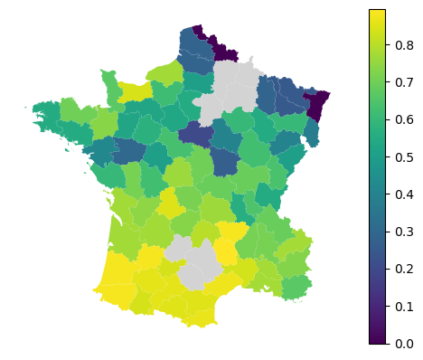
The local performance for such a model then looks like this.
local_f1 = model.local_metric(metrics.f1_score)

gdf.plot(local_f1, missing_kwds=dict(color='lightgray'), legend=True).set_axis_off()
Adapting the allowed proportion
The first thing you can do is to adapt the allowed minimum proportion. If you want to have less imbalanced models, you can increase it at the cost of more local models being skipped.
stricter_model = GWRandomForestClassifier(
    geometry=gdf.representative_point(),
    bandwidth=25,
    fixed=False,
    min_proportion=0.3
)
stricter_model.fit(
    X,
    y,
)
GWRandomForestClassifier(bandwidth=25,
                         geometry=0     POINT (827911.875 2122906.5)
1       POINT (691725.716 2496059)
2     POINT (663520.408 2152677.5)
3       POINT (908864.897 1915755)
4     POINT (916568.259 1968489.5)
                  ...
80      POINT (322806.903 2192566)
81      POINT (456440.882 2181291)
82     POINT (510125.65 2102842.5)
83      POINT (901963.264 2362015)
84       POINT (697522.96 2318253)
Length: 85, dtype: geometry,
                         min_proportion=0.3)
In a Jupyter environment, please rerun this cell to show the HTML representation or trust the notebook. On GitHub, the HTML representation is unable to render, please try loading this page with nbviewer.org.
Parameters
| bandwidth | 25 | |
| fixed | False | |
| kernel | 'bisquare' | |
| include_focal | False | |
| geometry | 0 POINT (...type: geometry | |
| graph | None | |
| n_jobs | -1 | |
| fit_global_model | True | |
| strict | False | |
| keep_models | False | |
| temp_folder | None | |
| batch_size | None | |
| min_proportion | 0.3 | |
| undersample | False | |
| leave_out | None | |
| random_state | None | |
| verbose | False |
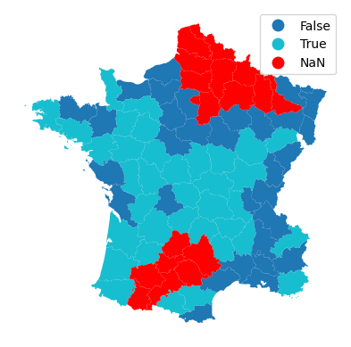
See how does that affect prediction rate.
stricter_model.prediction_rate_
np.float64(0.788235294117647)
About 12% less models can be fitted.
gdf.plot(stricter_model.pred_, missing_kwds=dict(color='red'), legend=True).set_axis_off()
Undersampling
Another strategy to battle with class imbalance, is to undersample data in each local model. By default, this is False, but can be set to True or a float. True ensured that both classes are equally represented, while float defines the minimum proportion of the minority class after resampling.
equal_model = GWRandomForestClassifier(
    geometry=gdf.representative_point(),
    bandwidth=25,
    fixed=False,
    min_proportion=0.3,
    undersample=True,
)
equal_model.fit(
    X,
    y,
)
GWRandomForestClassifier(bandwidth=25,
                         geometry=0     POINT (827911.875 2122906.5)
1       POINT (691725.716 2496059)
2     POINT (663520.408 2152677.5)
3       POINT (908864.897 1915755)
4     POINT (916568.259 1968489.5)
                  ...
80      POINT (322806.903 2192566)
81      POINT (456440.882 2181291)
82     POINT (510125.65 2102842.5)
83      POINT (901963.264 2362015)
84       POINT (697522.96 2318253)
Length: 85, dtype: geometry,
                         min_proportion=0.3, undersample=True)
In a Jupyter environment, please rerun this cell to show the HTML representation or trust the notebook. On GitHub, the HTML representation is unable to render, please try loading this page with nbviewer.org.
Parameters
| bandwidth | 25 | |
| fixed | False | |
| kernel | 'bisquare' | |
| include_focal | False | |
| geometry | 0 POINT (...type: geometry | |
| graph | None | |
| n_jobs | -1 | |
| fit_global_model | True | |
| strict | False | |
| keep_models | False | |
| temp_folder | None | |
| batch_size | None | |
| min_proportion | 0.3 | |
| undersample | True | |
| leave_out | None | |
| random_state | None | |
| verbose | False |
This does not affect the prediction rate.
equal_model.prediction_rate_
np.float64(0.788235294117647)
But does affect local, and hence global, performance of the model.
equal_f1 = equal_model.local_metric(metrics.f1_score)
stricter_f1 = stricter_model.local_metric(metrics.f1_score)

diff = equal_f1 - stricter_f1
See the difference in local F1 scores compared to a model without undersampling.
gdf.plot(diff, legend=True, missing_kwds=dict(color='red'), cmap='PiYG', vmax=np.nanmax(np.abs(diff))).set_axis_off()
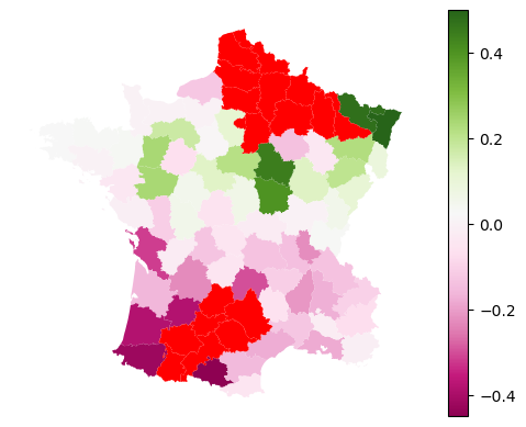
Keep in mind that for models like this one, where we use only 25 observations in each local model, undersampling can have a severe efect on the model robustness in a negative way, as it may reduce the number of observations that are actually used by quite a lot. Use with caution and ideally in situations where you rely on a larger number of neighbors.