Ensemble models
gwlearn currently implements geographically weighted versions of ensemble models for the classification tasks. However, there’s a caveat. Given it is unlikely that all categories are present in all local models, fitting a non-binary would lead to inconsistent local models. Hence gwlearn currently supports only binary classification.
import geopandas as gpd
from geodatasets import get_path
from sklearn import metrics

from gwlearn.ensemble import GWGradientBoostingClassifier, GWRandomForestClassifier
Get sample data
gdf = gpd.read_file(get_path("geoda.ncovr")).to_crs(5070)

gdf['point'] = gdf.representative_point()
gdf = gdf.set_geometry('point')

y = gdf["FH90"] > gdf["FH90"].median()
X = gdf.iloc[:, 9:15]
Random Forest
The implementation of geographically-weighted random forest classifier follows the logic of linear models, where each local neighborhood defiend by a set bandwidth is used to fit a single local model.
gwrf = GWRandomForestClassifier(
    geometry=gdf.geometry,
    bandwidth=250,
    fixed=False,
)
gwrf.fit(
    X,
    y,
)
GWRandomForestClassifier(bandwidth=250,
                         geometry=0          POINT (82374.171 2869835.025)
1       POINT (-1666267.814 3025996.603)
2        POINT (-1618645.796 3012447.96)
3       POINT (-1751938.544 3053013.371)
4       POINT (-1576454.985 3002625.267)
                      ...
3080    POINT (-1658725.535 1280845.161)
3081        POINT (-1089589 1376092.326)
3082     POINT (1700687.417 1750877.094)
3083     POINT (1588266.678 1896903.045)
3084    POINT (-1153940.634 2574551.428)
Name: point, Length: 3085, dtype: geometry)
In a Jupyter environment, please rerun this cell to show the HTML representation or trust the notebook. On GitHub, the HTML representation is unable to render, please try loading this page with nbviewer.org.
Parameters
| bandwidth | 250 | |
| fixed | False | |
| kernel | 'bisquare' | |
| include_focal | False | |
| geometry | 0 PO...type: geometry | |
| graph | None | |
| n_jobs | -1 | |
| fit_global_model | True | |
| strict | False | |
| keep_models | False | |
| temp_folder | None | |
| batch_size | None | |
| min_proportion | 0.2 | |
| undersample | False | |
| leave_out | None | |
| random_state | None | |
| verbose | False |
Focal score
The performance of these models can be measured in three ways. The first one is using the focal prediction. Unlike in linear models, where the focal observation is part of the local model training, in this case it is excluded to ensure it can be used to evaluate the model. Otherwise, it would be a part of the data the local model has seen and would report unrealistically high performance. If you want to include the focal observation in the training nevertheless, just set include_focal=True.
Focal accuracy can be measured as follows. Note that some local models are not fitted due to imbalance rules, and report NA that needs to be filtered out.
na_mask = gwrf.pred_.notna()

metrics.accuracy_score(y[na_mask], gwrf.pred_[na_mask])
0.7635574837310195
Pooled out-of-bag score
Another option is to pull the out-of-bag predictions from individual local models and pool them together. This uses more data to evaluate the model but given the local models are tuned for their focal location, some predictions on locations far from the focal point may be artifically worse than the actual model prediction would be.
metrics.accuracy_score(gwrf.oob_y_pooled_, gwrf.oob_pred_pooled_)
0.7639566160520608
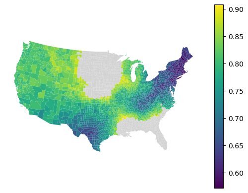
Local score
The final option is to take the local out-of-bag predicitons and measure performance per each local model. To do that, you can use a method local_metric().
local_accuracy = gwrf.local_metric(metrics.accuracy_score)
local_accuracy
array([ nan, 0.812, 0.824, ..., 0.732, 0.704, 0.848], shape=(3085,))
gdf.set_geometry('geometry').plot(local_accuracy, legend=True, missing_kwds=dict(color='lightgray')).set_axis_off()
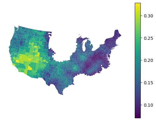
Feature importance
Feature importances are reported for each local model.
gwrf.feature_importances_
| HR60 | HR70 | HR80 | HR90 | HC60 | HC70 | |
|---|---|---|---|---|---|---|
| 0 | NaN | NaN | NaN | NaN | NaN | NaN |
| 1 | 0.179267 | 0.139123 | 0.124227 | 0.160139 | 0.197307 | 0.199936 |
| 2 | 0.178505 | 0.136469 | 0.130985 | 0.170816 | 0.168485 | 0.214740 |
| 3 | 0.144078 | 0.133436 | 0.129812 | 0.165222 | 0.165138 | 0.262315 |
| 4 | 0.149554 | 0.142001 | 0.118353 | 0.160402 | 0.182540 | 0.247150 |
| ... | ... | ... | ... | ... | ... | ... |
| 3080 | 0.145577 | 0.092096 | 0.202522 | 0.097916 | 0.290165 | 0.171724 |
| 3081 | 0.145981 | 0.096929 | 0.158639 | 0.198414 | 0.234700 | 0.165337 |
| 3082 | 0.143242 | 0.215822 | 0.186652 | 0.222352 | 0.094151 | 0.137781 |
| 3083 | 0.161037 | 0.167594 | 0.188477 | 0.266096 | 0.092027 | 0.124768 |
| 3084 | 0.096781 | 0.129547 | 0.160739 | 0.189850 | 0.213452 | 0.209630 |
3085 rows × 6 columns
gdf.set_geometry('geometry').plot(gwrf.feature_importances_["HC60"], legend=True).set_axis_off()
You can compare all of this to values extracted from a global model, fitted alongside.
gwrf.global_model.feature_importances_
array([0.13568658, 0.14795968, 0.18836118, 0.20578669, 0.14827197,
       0.17393389])
gwrf.feature_importances_.mean()
HR60    0.142798
HR70    0.156280
HR80    0.189687
HR90    0.191350
HC60    0.146587
HC70    0.173299
dtype: float64
Gradient boosting
If you prefer to use gradient boosting, there is a minimal implementation of geographically weighted gradient boosting classifier, following the same model described for the random forest above.
gwgb = GWGradientBoostingClassifier(
    geometry=gdf.geometry,
    bandwidth=250,
    fixed=False,
)
gwgb.fit(
    X,
    y,
)
GWGradientBoostingClassifier(bandwidth=250,
                             geometry=0          POINT (82374.171 2869835.025)
1       POINT (-1666267.814 3025996.603)
2        POINT (-1618645.796 3012447.96)
3       POINT (-1751938.544 3053013.371)
4       POINT (-1576454.985 3002625.267)
                      ...
3080    POINT (-1658725.535 1280845.161)
3081        POINT (-1089589 1376092.326)
3082     POINT (1700687.417 1750877.094)
3083     POINT (1588266.678 1896903.045)
3084    POINT (-1153940.634 2574551.428)
Name: point, Length: 3085, dtype: geometry)
In a Jupyter environment, please rerun this cell to show the HTML representation or trust the notebook. On GitHub, the HTML representation is unable to render, please try loading this page with nbviewer.org.
Parameters
| bandwidth | 250 | |
| fixed | False | |
| kernel | 'bisquare' | |
| include_focal | False | |
| geometry | 0 PO...type: geometry | |
| graph | None | |
| n_jobs | -1 | |
| fit_global_model | True | |
| strict | False | |
| keep_models | False | |
| temp_folder | None | |
| batch_size | None |
Given the nature of the model, the outputs are a bit more limited. You can still extract focal predictions.
nan_mask = gwgb.pred_.notna()

metrics.accuracy_score(y[nan_mask], gwgb.pred_[nan_mask])
0.7483731019522777
And local feature importances.
gwgb.feature_importances_
| HR60 | HR70 | HR80 | HR90 | HC60 | HC70 | |
|---|---|---|---|---|---|---|
| 0 | NaN | NaN | NaN | NaN | NaN | NaN |
| 1 | 0.173350 | 0.122193 | 0.066879 | 0.161867 | 0.134879 | 0.340832 |
| 2 | 0.189628 | 0.122011 | 0.063924 | 0.163806 | 0.118613 | 0.342017 |
| 3 | 0.146307 | 0.139012 | 0.077630 | 0.170284 | 0.071027 | 0.395741 |
| 4 | 0.166607 | 0.133140 | 0.072732 | 0.159727 | 0.111422 | 0.356372 |
| ... | ... | ... | ... | ... | ... | ... |
| 3080 | 0.099314 | 0.056185 | 0.143100 | 0.045828 | 0.592708 | 0.062865 |
| 3081 | 0.088293 | 0.067453 | 0.139627 | 0.227565 | 0.442186 | 0.034876 |
| 3082 | 0.101723 | 0.190659 | 0.173942 | 0.335706 | 0.063783 | 0.134187 |
| 3083 | 0.136217 | 0.164555 | 0.158056 | 0.363580 | 0.047310 | 0.130281 |
| 3084 | 0.028864 | 0.100108 | 0.098761 | 0.224582 | 0.430143 | 0.117543 |
3085 rows × 6 columns
Leave out samples
However, the pooled data are not available. In this case, you can use the leave_out keyword to leave out a fraction (when float) or a set number (when int) of random observations from each local model. For these, the local model does prediction and returns as left_out_proba_ and left_out_y_ arrays.
gwgb_leave = GWGradientBoostingClassifier(
    geometry=gdf.geometry,
    bandwidth=250,
    fixed=False,
    leave_out=.2
)
gwgb_leave.fit(
    X,
    y,
)
GWGradientBoostingClassifier(bandwidth=250,
                             geometry=0          POINT (82374.171 2869835.025)
1       POINT (-1666267.814 3025996.603)
2        POINT (-1618645.796 3012447.96)
3       POINT (-1751938.544 3053013.371)
4       POINT (-1576454.985 3002625.267)
                      ...
3080    POINT (-1658725.535 1280845.161)
3081        POINT (-1089589 1376092.326)
3082     POINT (1700687.417 1750877.094)
3083     POINT (1588266.678 1896903.045)
3084    POINT (-1153940.634 2574551.428)
Name: point, Length: 3085, dtype: geometry)
In a Jupyter environment, please rerun this cell to show the HTML representation or trust the notebook. On GitHub, the HTML representation is unable to render, please try loading this page with nbviewer.org.
Parameters
| bandwidth | 250 | |
| fixed | False | |
| kernel | 'bisquare' | |
| include_focal | False | |
| geometry | 0 PO...type: geometry | |
| graph | None | |
| n_jobs | -1 | |
| fit_global_model | True | |
| strict | False | |
| keep_models | False | |
| temp_folder | None | |
| batch_size | None |
metrics.accuracy_score(gwgb_leave.left_out_y_, gwgb_leave.left_out_proba_.argmax(axis=1))
0.7502559652928417