This page was generated from notebooks/RankMarkov.ipynb. Interactive online version:

Full Rank Markov and Geographic Rank Markov¶

Author: Wei Kang weikang9009@gmail.com

[1]:

import warnings

with warnings.catch_warnings():
    warnings.simplefilter("ignore")
    # ignore NumbaDeprecationWarning: gh-pysal/libpysal#560
    import libpysal as ps

import numpy as np
import matplotlib.pyplot as plt
import seaborn as sns
import pandas as pd
import geopandas as gpd

Full Rank Markov¶

[2]:

with warnings.catch_warnings():
    warnings.simplefilter("ignore")
    # ignore NumbaDeprecationWarning: gh-pysal/libpysal#560
    from giddy.markov import FullRank_Markov

[3]:

income_table = pd.read_csv(ps.examples.get_path("usjoin.csv"))
income_table.head()

[3]:

	Name	STATE_FIPS	1929	1930	1931	1932	1933	1934	1935	1936	...	2000	2001	2002	2003	2004	2005	2006	2007	2008	2009
0	Alabama	1	323	267	224	162	166	211	217	251	...	23471	24467	25161	26065	27665	29097	30634	31988	32819	32274
1	Arizona	4	600	520	429	321	308	362	416	462	...	25578	26232	26469	27106	28753	30671	32552	33470	33445	32077
2	Arkansas	5	310	228	215	157	157	187	207	247	...	22257	23532	23929	25074	26465	27512	29041	31070	31800	31493
3	California	6	991	887	749	580	546	603	660	771	...	32275	32750	32900	33801	35663	37463	40169	41943	42377	40902
4	Colorado	8	634	578	471	354	353	368	444	542	...	32949	34228	33963	34092	35543	37388	39662	41165	41719	40093

5 rows × 83 columns

[4]:

pci = income_table[list(map(str, range(1929, 2010)))].values
pci

[4]:

array([[  323,   267,   224, ..., 31988, 32819, 32274],
       [  600,   520,   429, ..., 33470, 33445, 32077],
       [  310,   228,   215, ..., 31070, 31800, 31493],
       ...,
       [  460,   408,   356, ..., 29769, 31265, 31843],
       [  673,   588,   469, ..., 35839, 36594, 35676],
       [  675,   585,   476, ..., 43453, 45177, 42504]])

[5]:

m = FullRank_Markov(pci)
m.ranks

The Markov Chain is irreducible and is composed by:
1 Recurrent class (indices):
[ 0  1  2  3  4  5  6  7  8  9 10 11 12 13 14 15 16 17 18 19 20 21 22 23
 24 25 26 27 28 29 30 31 32 33 34 35 36 37 38 39 40 41 42 43 44 45 46 47]
0 Transient classes.
The Markov Chain has 0 absorbing states.

[5]:

array([[45, 45, 44, ..., 41, 40, 39],
       [24, 25, 25, ..., 36, 38, 41],
       [46, 47, 45, ..., 43, 43, 43],
       ...,
       [34, 34, 34, ..., 47, 46, 42],
       [17, 17, 22, ..., 25, 26, 25],
       [16, 18, 19, ...,  6,  6,  7]])

[6]:

m.transitions

[6]:

array([[66.,  5.,  5., ...,  0.,  0.,  0.],
       [ 8., 51.,  9., ...,  0.,  0.,  0.],
       [ 2., 13., 44., ...,  0.,  0.,  0.],
       ...,
       [ 0.,  0.,  0., ..., 40., 17.,  0.],
       [ 0.,  0.,  0., ..., 15., 54.,  2.],
       [ 0.,  0.,  0., ...,  2.,  1., 77.]])

Full rank Markov transition probability matrix

[7]:

m.p

[7]:

array([[0.825 , 0.0625, 0.0625, ..., 0.    , 0.    , 0.    ],
       [0.1   , 0.6375, 0.1125, ..., 0.    , 0.    , 0.    ],
       [0.025 , 0.1625, 0.55  , ..., 0.    , 0.    , 0.    ],
       ...,
       [0.    , 0.    , 0.    , ..., 0.5   , 0.2125, 0.    ],
       [0.    , 0.    , 0.    , ..., 0.1875, 0.675 , 0.025 ],
       [0.    , 0.    , 0.    , ..., 0.025 , 0.0125, 0.9625]])

Full rank mean first passage times

[8]:

m.mfpt

[8]:

array([[  48.        ,   87.96280048,   68.1089084 , ...,  443.76689275,
         518.31000749, 1628.59025557],
       [ 225.92564594,   48.        ,   78.75804364, ...,  440.0173313 ,
         514.56045127, 1624.84070661],
       [ 271.55443692,  102.484092  ,   48.        , ...,  438.93288204,
         513.47599512, 1623.75624059],
       ...,
       [ 727.11189921,  570.15910508,  546.61934646, ...,   48.        ,
         117.41906375, 1278.96860316],
       [ 730.40467469,  573.45179415,  549.91216045, ...,   49.70722573,
          48.        , 1202.06279368],
       [ 754.8761577 ,  597.92333477,  574.38361779, ...,   43.23574191,
         104.9460425 ,   48.        ]])

[9]:

m.sojourn_time

[9]:

array([ 5.71428571,  2.75862069,  2.22222222,  1.77777778,  1.66666667,
        1.73913043,  1.53846154,  1.53846154,  1.53846154,  1.42857143,
        1.42857143,  1.56862745,  1.53846154,  1.40350877,  1.29032258,
        1.21212121,  1.31147541,  1.37931034,  1.29032258,  1.25      ,
        1.15942029,  1.12676056,  1.25      ,  1.17647059,  1.19402985,
        1.08108108,  1.19402985,  1.25      ,  1.25      ,  1.14285714,
        1.33333333,  1.26984127,  1.25      ,  1.37931034,  1.42857143,
        1.31147541,  1.26984127,  1.25      ,  1.31147541,  1.25      ,
        1.19402985,  1.25      ,  1.53846154,  1.6       ,  1.86046512,
        2.        ,  3.07692308, 26.66666667])

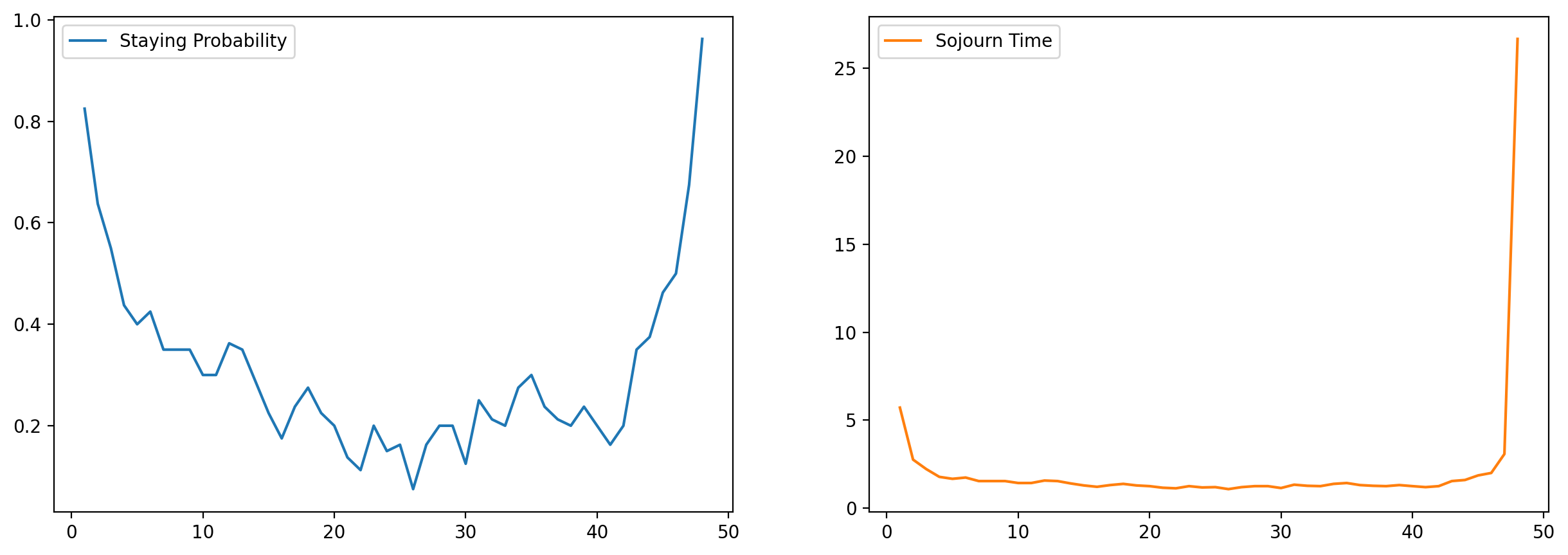
[10]:

df_fullrank = pd.DataFrame(
    np.c_[m.p.diagonal(), m.sojourn_time],
    columns=["Staying Probability", "Sojourn Time"],
    index=np.arange(m.p.shape[0]) + 1,
)
df_fullrank.head()

[10]:

	Staying Probability	Sojourn Time
1	0.8250	5.714286
2	0.6375	2.758621
3	0.5500	2.222222
4	0.4375	1.777778
5	0.4000	1.666667

[11]:

df_fullrank.plot(subplots=True, layout=(1, 2), figsize=(15, 5))

[11]:

array([[<Axes: >, <Axes: >]], dtype=object)

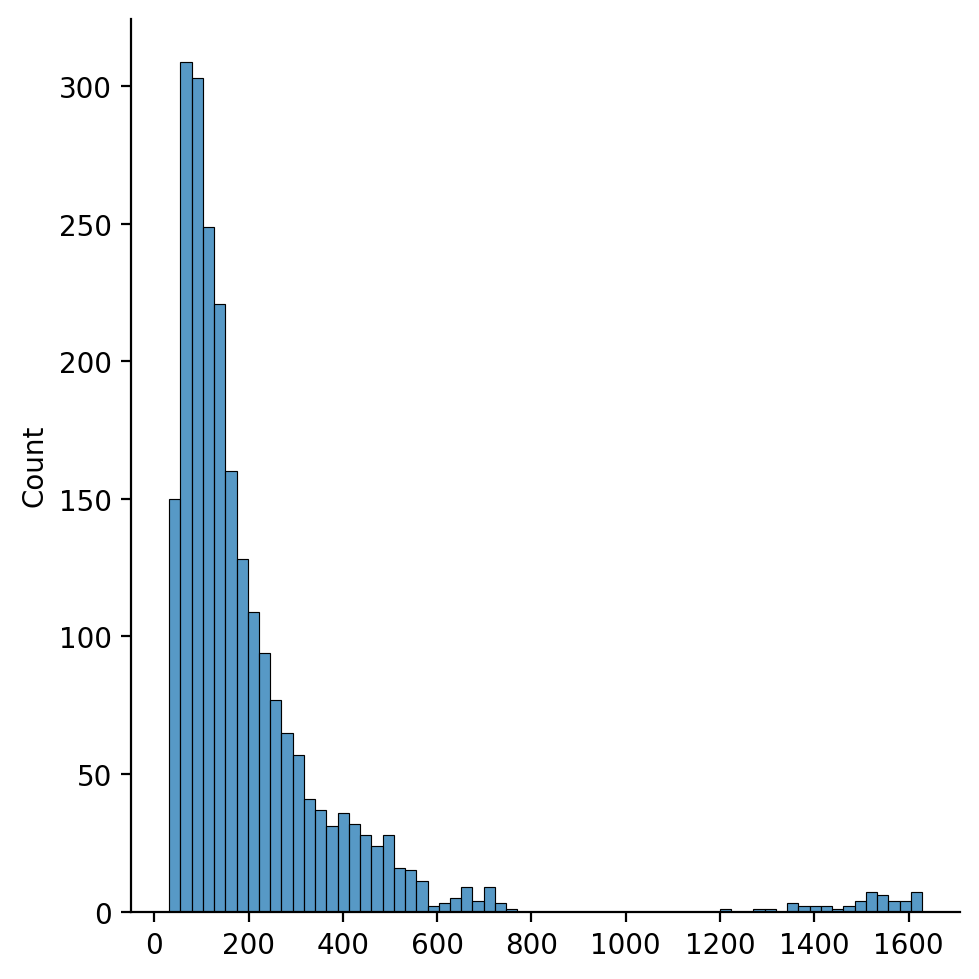
../_images/notebooks_RankMarkov_14_1.png

[12]:

with warnings.catch_warnings():
    warnings.simplefilter("ignore")
    # ignore -- seaborn/_oldcore.py:1498: FutureWarning: is_categorical_dtype is deprecated
    # and will be removed in a future version. Use isinstance(dtype, CategoricalDtype) instead

    # ignore -- seaborn/_oldcore.py:1119: FutureWarning: use_inf_as_na option is deprecated
    # and will be removed in a future version. Convert inf values to NaN before operating instead.

    sns.displot(m.mfpt.flatten(), kde=False)

../_images/notebooks_RankMarkov_15_0.png

Geographic Rank Markov¶

[13]:

from giddy.markov import GeoRank_Markov, Markov, sojourn_time

gm = GeoRank_Markov(pci)

The Markov Chain is irreducible and is composed by:
1 Recurrent class (indices):
[ 0  1  2  3  4  5  6  7  8  9 10 11 12 13 14 15 16 17 18 19 20 21 22 23
 24 25 26 27 28 29 30 31 32 33 34 35 36 37 38 39 40 41 42 43 44 45 46 47]
0 Transient classes.
The Markov Chain has 0 absorbing states.

[14]:

gm.transitions

[14]:

array([[38.,  0.,  8., ...,  0.,  0.,  0.],
       [ 0., 15.,  0., ...,  0.,  1.,  0.],
       [ 6.,  0., 44., ...,  5.,  0.,  0.],
       ...,
       [ 2.,  0.,  5., ..., 34.,  0.,  0.],
       [ 0.,  0.,  0., ...,  0., 18.,  2.],
       [ 0.,  0.,  0., ...,  0.,  3., 14.]])

[15]:

gm.p

[15]:

array([[0.475 , 0.    , 0.1   , ..., 0.    , 0.    , 0.    ],
       [0.    , 0.1875, 0.    , ..., 0.    , 0.0125, 0.    ],
       [0.075 , 0.    , 0.55  , ..., 0.0625, 0.    , 0.    ],
       ...,
       [0.025 , 0.    , 0.0625, ..., 0.425 , 0.    , 0.    ],
       [0.    , 0.    , 0.    , ..., 0.    , 0.225 , 0.025 ],
       [0.    , 0.    , 0.    , ..., 0.    , 0.0375, 0.175 ]])

[16]:

gm.sojourn_time[:10]

[16]:

array([1.9047619 , 1.23076923, 2.22222222, 1.73913043, 1.15942029,
       3.80952381, 1.70212766, 1.25      , 1.31147541, 1.11111111])

[17]:

gm.sojourn_time

[17]:

array([ 1.9047619 ,  1.23076923,  2.22222222,  1.73913043,  1.15942029,
        3.80952381,  1.70212766,  1.25      ,  1.31147541,  1.11111111,
        1.73913043,  1.37931034,  1.17647059,  1.21212121,  1.33333333,
        1.37931034,  1.09589041,  2.10526316,  2.        ,  1.45454545,
        1.26984127, 26.66666667,  1.19402985,  1.23076923,  1.09589041,
        1.56862745,  1.26984127,  2.42424242,  1.50943396,  2.        ,
        1.29032258,  1.09589041,  1.6       ,  1.42857143,  1.25      ,
        1.45454545,  1.29032258,  1.6       ,  1.17647059,  1.56862745,
        1.25      ,  1.37931034,  1.45454545,  1.42857143,  1.29032258,
        1.73913043,  1.29032258,  1.21212121])

[18]:

gm.mfpt

[18]:

array([[ 48.        ,  63.35532038,  92.75274652, ...,  82.47515731,
         71.01114491,  68.65737127],
       [108.25928005,  48.        , 127.99032986, ...,  92.03098299,
         63.36652935,  61.82733039],
       [ 76.96801786,  64.7713783 ,  48.        , ...,  73.84595169,
         72.24682723,  69.77497173],
       ...,
       [ 93.3107474 ,  62.47670463, 105.80634118, ...,  48.        ,
         69.30121319,  67.08838421],
       [113.65278078,  61.1987031 , 133.57991745, ...,  96.0103924 ,
         48.        ,  56.74165107],
       [114.71894813,  63.4019776 , 134.73381719, ...,  97.287895  ,
         61.45565054,  48.        ]])

[19]:

income_table["geo_sojourn_time"] = gm.sojourn_time
i = 0
for state in income_table["Name"]:
    income_table[f"geo_mfpt_to_{state}"] = gm.mfpt[:, i]
    income_table[f"geo_mfpt_from_{state}"] = gm.mfpt[i, :]
    i = i + 1
income_table.head()

[19]:

	Name	STATE_FIPS	1929	1930	1931	1932	1933	1934	1935	1936	...	geo_mfpt_to_Virginia	geo_mfpt_from_Virginia	geo_mfpt_to_Washington	geo_mfpt_from_Washington	geo_mfpt_to_West Virginia	geo_mfpt_from_West Virginia	geo_mfpt_to_Wisconsin	geo_mfpt_from_Wisconsin	geo_mfpt_to_Wyoming	geo_mfpt_from_Wyoming
0	Alabama	1	323	267	224	162	166	211	217	251	...	72.186055	109.828532	82.994754	118.769984	82.475157	93.310747	71.011145	113.652781	68.657371	114.718948
1	Arizona	4	600	520	429	321	308	362	416	462	...	67.544447	60.838807	76.090895	66.729262	92.030983	62.476705	63.366529	61.198703	61.827330	63.401978
2	Arkansas	5	310	228	215	157	157	187	207	247	...	73.650943	129.533691	84.071211	138.692513	73.845952	105.806341	72.246827	133.579917	69.774972	134.733817
3	California	6	991	887	749	580	546	603	660	771	...	71.377700	111.644884	62.230417	97.908341	104.922271	121.670243	69.368408	110.668388	59.998457	105.965215
4	Colorado	8	634	578	471	354	353	368	444	542	...	69.627179	57.106339	66.353930	52.229230	98.797636	66.464398	60.762589	52.324565	55.559020	53.872702

5 rows × 180 columns

[20]:

geo_table = gpd.read_file(ps.examples.get_path("us48.shp"))
complete_table = geo_table.merge(income_table, left_on="STATE_NAME", right_on="Name")
complete_table.head()

[20]:

	AREA	PERIMETER	STATE_	STATE_ID	STATE_NAME	STATE_FIPS_x	SUB_REGION	STATE_ABBR	geometry	Name	...	geo_mfpt_to_Virginia	geo_mfpt_from_Virginia	geo_mfpt_to_Washington	geo_mfpt_from_Washington	geo_mfpt_to_West Virginia	geo_mfpt_from_West Virginia	geo_mfpt_to_Wisconsin	geo_mfpt_from_Wisconsin	geo_mfpt_to_Wyoming	geo_mfpt_from_Wyoming
0	20.750	34.956	1	1	Washington	53	Pacific	WA	MULTIPOLYGON (((-122.40075 48.22540, -122.4615...	Washington	...	71.663055	73.756804	48.000000	48.000000	101.592400	81.692586	65.219124	70.701226	53.126177	64.476985
1	45.132	34.527	2	2	Montana	30	Mtn	MT	POLYGON ((-111.47463 44.70224, -111.48001 44.6...	Montana	...	69.918931	59.067897	76.184088	64.710823	90.781850	58.795201	63.455248	58.975522	60.881954	60.553000
2	9.571	18.899	3	3	Maine	23	N Eng	ME	MULTIPOLYGON (((-69.77779 44.07407, -69.86044 ...	Maine	...	69.431862	53.872836	77.512381	62.862378	87.734760	54.244823	66.257807	56.905741	61.978506	58.336426
3	21.874	21.353	4	4	North Dakota	38	W N Cen	ND	POLYGON ((-98.73006 45.93830, -99.00645 45.939...	North Dakota	...	69.441690	56.526347	76.659646	62.823668	85.031218	49.511240	67.362718	58.717458	64.386382	59.728719
4	22.598	22.746	5	5	South Dakota	46	W N Cen	SD	POLYGON ((-102.78793 42.99532, -103.00541 42.9...	South Dakota	...	68.229894	61.548209	78.886304	68.794083	88.192659	55.754109	66.187694	63.802359	64.336311	65.070022

5 rows × 189 columns

[21]:

complete_table.columns

[21]:

Index(['AREA', 'PERIMETER', 'STATE_', 'STATE_ID', 'STATE_NAME', 'STATE_FIPS_x',
       'SUB_REGION', 'STATE_ABBR', 'geometry', 'Name',
       ...
       'geo_mfpt_to_Virginia', 'geo_mfpt_from_Virginia',
       'geo_mfpt_to_Washington', 'geo_mfpt_from_Washington',
       'geo_mfpt_to_West Virginia', 'geo_mfpt_from_West Virginia',
       'geo_mfpt_to_Wisconsin', 'geo_mfpt_from_Wisconsin',
       'geo_mfpt_to_Wyoming', 'geo_mfpt_from_Wyoming'],
      dtype='object', length=189)

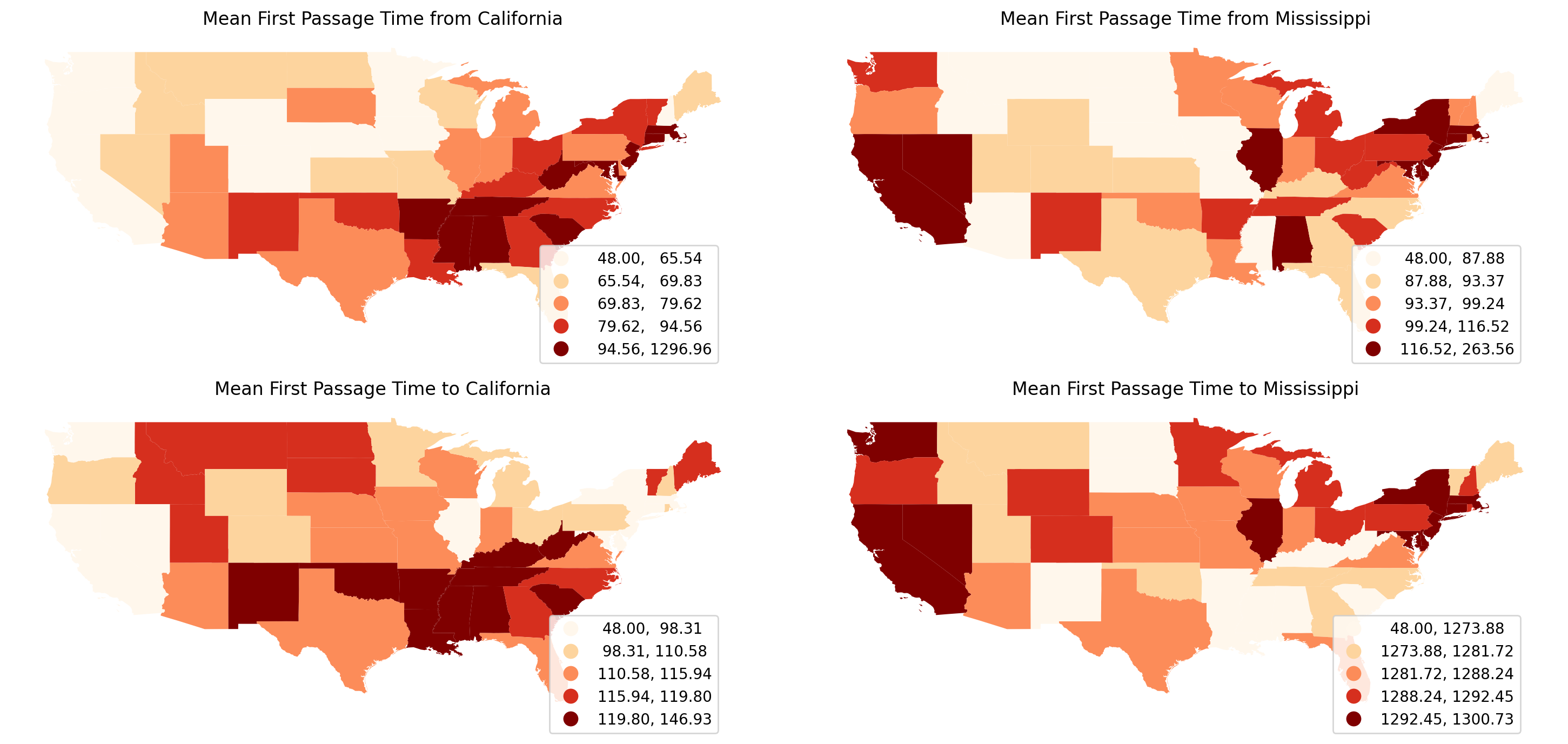
Visualizing mean first passage time from/to California/Mississippi:

[22]:

with warnings.catch_warnings():
    warnings.simplefilter("ignore")
    # ignore geopandas/plotting.py:732:
    # FutureWarning: is_categorical_dtype is deprecated and will be removed in a future version.

    fig, axes = plt.subplots(nrows=2, ncols=2, figsize=(15, 7))
    target_states = ["California", "Mississippi"]
    directions = ["from", "to"]
    plt_kws = dict(cmap="OrRd", scheme="quantiles", legend=True)
    for i, direction in enumerate(directions):
        for j, target in enumerate(target_states):
            ax = axes[i, j]
            col = f"{direction}_{target}"
            complete_table.plot(ax=ax, column=f"geo_mfpt_{col}", **plt_kws)
            ax.set_title(f"Mean First Passage Time {direction} {target}")
            ax.axis("off")
            leg = ax.get_legend()
            leg.set_bbox_to_anchor((0.8, 0.15, 0.16, 0.2))
    plt.tight_layout()

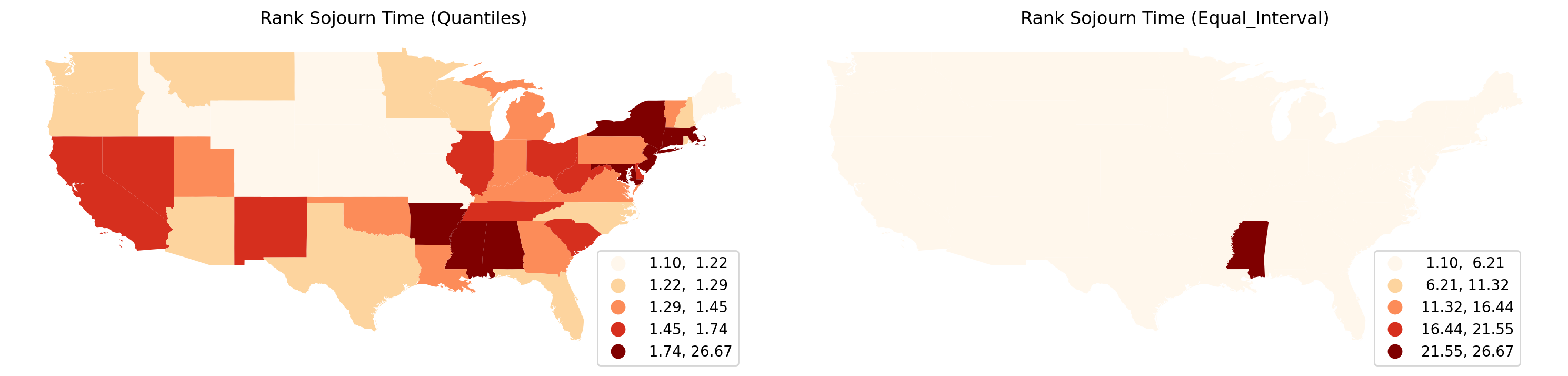
../_images/notebooks_RankMarkov_27_0.png

Visualizing sojourn time for each US state:

[23]:

with warnings.catch_warnings():
    warnings.simplefilter("ignore")
    # ignore geopandas/plotting.py:732:
    # FutureWarning: is_categorical_dtype is deprecated and will be removed in a future version.

    fig, axes = plt.subplots(nrows=1, ncols=2, figsize=(15, 7))
    schemes = ["Quantiles", "Equal_Interval"]
    plt_kws = dict(cmap="OrRd", legend=True, column="geo_sojourn_time")
    for i, scheme in enumerate(schemes):
        ax = axes[i]
        complete_table.plot(ax=ax, scheme=scheme, **plt_kws)
        ax.set_title(f"Rank Sojourn Time ({scheme})")
        ax.axis("off")
        leg = ax.get_legend()
        leg.set_bbox_to_anchor((0.8, 0.15, 0.16, 0.2))
    plt.tight_layout()

../_images/notebooks_RankMarkov_29_0.png