This page was generated from notebooks/08_manual_coloring.ipynb.
Interactive online version:
![]()
[1]:
import geodatasets
import geopandas as gpd
import pandas as pd

import mapclassify
from mapclassify.util import get_color_array

%load_ext watermark
%watermark -a 'eli knaap' -iv
Author: eli knaap

pandas     : 2.3.1
geodatasets: 2024.8.0
geopandas  : 1.1.1
mapclassify: 2.9.1.dev9+gde74d6f.d20250614
[2]:
df = gpd.read_file(geodatasets.get_path("geoda cincinnati")).to_crs(4326)
[3]:
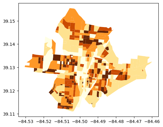
# use mapclassify under the hood
df.plot("DENSITY", scheme="quantiles", cmap="YlOrBr")
[3]:
<Axes: >

[4]:
# get colors directly and pass them to geopandas
colors = get_color_array(
    df.DENSITY.values, scheme="quantiles", cmap="YlOrBr", as_hex=True
)
[5]:
colors
[5]:
array(['#fee290', '#fd9828', '#fee290', '#662505', '#fee290', '#fd9828',
       '#662505', '#fd9828', '#fd9828', '#ca4b02', '#fd9828', '#662505',
       '#662505', '#fd9828', '#ffffe5', '#662505', '#662505', '#ca4b02',
       '#662505', '#662505', '#fee290', '#662505', '#ca4b02', '#662505',
       '#ffffe5', '#fd9828', '#fee290', '#ca4b02', '#fd9828', '#fd9828',
       '#ffffe5', '#ca4b02', '#fd9828', '#ca4b02', '#ffffe5', '#662505',
       '#662505', '#ca4b02', '#fd9828', '#ca4b02', '#fee290', '#ca4b02',
       '#662505', '#ffffe5', '#fd9828', '#fd9828', '#fd9828', '#fee290',
       '#fee290', '#fee290', '#662505', '#ffffe5', '#ffffe5', '#fee290',
       '#ffffe5', '#ca4b02', '#fd9828', '#fd9828', '#ffffe5', '#ca4b02',
       '#fd9828', '#fee290', '#ca4b02', '#ca4b02', '#ca4b02', '#ca4b02',
       '#662505', '#fd9828', '#fee290', '#fee290', '#fee290', '#fee290',
       '#fee290', '#ffffe5', '#fd9828', '#ffffe5', '#ffffe5', '#fee290',
       '#fd9828', '#ffffe5', '#ffffe5', '#ffffe5', '#ffffe5', '#ffffe5',
       '#ffffe5', '#fee290', '#ffffe5', '#fee290', '#ca4b02', '#ffffe5',
       '#ffffe5', '#ffffe5', '#ca4b02', '#fee290', '#ffffe5', '#662505',
       '#662505', '#fee290', '#fd9828', '#ffffe5', '#ca4b02', '#ffffe5',
       '#fd9828', '#fd9828', '#662505', '#662505', '#fd9828', '#fee290',
       '#fd9828', '#662505', '#fd9828', '#ffffe5', '#ca4b02', '#fd9828',
       '#662505', '#ca4b02', '#662505', '#fd9828', '#fee290', '#ca4b02',
       '#fee290', '#ffffe5', '#ffffe5', '#ffffe5', '#fd9828', '#662505',
       '#ca4b02', '#ffffe5', '#fd9828', '#fee290', '#ffffe5', '#ca4b02',
       '#ffffe5', '#fee290', '#fee290', '#ffffe5', '#662505', '#ffffe5',
       '#fd9828', '#662505', '#fd9828', '#662505', '#662505', '#ffffe5',
       '#662505', '#ffffe5', '#662505', '#ffffe5', '#fd9828', '#ffffe5',
       '#ffffe5', '#ca4b02', '#662505', '#662505', '#ca4b02', '#662505',
       '#ffffe5', '#662505', '#ca4b02', '#fee290', '#fd9828', '#ca4b02',
       '#662505', '#ffffe5', '#fd9828', '#fd9828', '#ca4b02', '#ca4b02',
       '#662505', '#ffffe5', '#fee290', '#fee290', '#662505', '#ca4b02',
       '#ffffe5', '#662505', '#fd9828', '#fd9828', '#ffffe5', '#ffffe5',
       '#fee290', '#fee290', '#fee290', '#ffffe5', '#ffffe5', '#fee290',
       '#ffffe5', '#ffffe5', '#ffffe5', '#ffffe5', '#ca4b02', '#ffffe5',
       '#fee290', '#ffffe5', '#662505', '#fee290', '#fee290', '#662505',
       '#fd9828', '#fd9828', '#ca4b02', '#ca4b02', '#ffffe5', '#fee290',
       '#fee290', '#662505', '#ffffe5', '#fd9828', '#ffffe5', '#ffffe5',
       '#fee290', '#fd9828', '#fd9828', '#fee290', '#ca4b02', '#ca4b02',
       '#fd9828', '#fee290', '#fee290', '#fee290', '#fee290', '#fee290',
       '#fee290', '#ca4b02', '#fee290', '#662505', '#fee290', '#662505',
       '#ca4b02', '#662505', '#662505', '#fd9828', '#ffffe5', '#ffffe5',
       '#ffffe5', '#ffffe5', '#ca4b02', '#662505', '#ca4b02', '#662505',
       '#662505', '#ffffe5', '#ffffe5', '#ca4b02', '#ca4b02', '#ca4b02',
       '#ca4b02', '#ca4b02', '#662505', '#ffffe5', '#fee290', '#fee290',
       '#fee290', '#ffffe5', '#fee290', '#ffffe5', '#ffffe5', '#fee290',
       '#fee290', '#fee290', '#ca4b02', '#662505', '#fd9828', '#fd9828',
       '#662505', '#fd9828', '#ca4b02', '#ffffe5', '#662505', '#fd9828',
       '#fee290', '#ffffe5', '#fee290', '#ca4b02', '#ca4b02', '#ca4b02',
       '#ca4b02', '#fd9828', '#fd9828', '#662505', '#ca4b02', '#ca4b02',
       '#ca4b02', '#ca4b02', '#ca4b02', '#fd9828', '#fd9828', '#ca4b02',
       '#662505', '#ca4b02', '#662505', '#ca4b02', '#ca4b02', '#ca4b02',
       '#fee290', '#ffffe5', '#ffffe5', '#662505', '#ca4b02', '#fee290',
       '#fee290', '#ffffe5', '#fd9828', '#ca4b02', '#fd9828', '#fd9828',
       '#fee290', '#fee290', '#662505', '#fd9828', '#ca4b02', '#ffffe5',
       '#fee290', '#fee290', '#662505', '#662505', '#ffffe5', '#662505',
       '#662505', '#ca4b02', '#fee290', '#fd9828', '#fee290', '#662505',
       '#ffffe5', '#662505', '#ffffe5', '#ffffe5', '#ffffe5', '#fee290',
       '#ffffe5', '#ffffe5', '#fee290', '#ffffe5', '#fd9828', '#fee290',
       '#662505', '#ffffe5', '#fee290', '#ffffe5', '#662505', '#ffffe5',
       '#ffffe5', '#fee290', '#ca4b02', '#fd9828', '#fee290', '#fd9828',
       '#fee290', '#662505', '#fee290', '#662505', '#fd9828', '#662505',
       '#662505', '#fd9828', '#fee290', '#fd9828', '#662505', '#662505',
       '#fee290', '#fd9828', '#ca4b02', '#fd9828', '#ffffe5', '#fee290',
       '#ca4b02', '#ca4b02', '#fee290', '#ffffe5', '#fd9828', '#fee290',
       '#fd9828', '#ffffe5', '#662505', '#fee290', '#fd9828', '#fee290',
       '#ca4b02', '#ffffe5', '#fd9828', '#662505', '#fd9828', '#ca4b02',
       '#662505', '#662505', '#fd9828', '#662505', '#662505', '#662505',
       '#ca4b02', '#fd9828', '#fee290', '#fee290', '#ca4b02', '#ffffe5',
       '#662505', '#fd9828', '#ca4b02', '#662505', '#ca4b02', '#ffffe5',
       '#ca4b02', '#662505', '#ca4b02', '#662505', '#662505', '#ca4b02',
       '#ca4b02', '#fd9828', '#662505', '#fd9828', '#fee290', '#662505',
       '#662505', '#662505', '#fee290', '#fd9828', '#ca4b02', '#fee290',
       '#ca4b02', '#662505', '#fd9828', '#fd9828', '#ca4b02', '#662505',
       '#fd9828', '#fd9828', '#fee290', '#ca4b02', '#fd9828', '#ca4b02',
       '#ca4b02', '#ca4b02', '#fd9828', '#ca4b02', '#fd9828', '#ca4b02',
       '#ca4b02', '#ca4b02', '#fd9828', '#fd9828', '#fd9828', '#662505',
       '#fee290', '#ca4b02', '#fd9828', '#fee290', '#662505', '#662505',
       '#fd9828', '#662505', '#fd9828', '#fd9828', '#ffffe5', '#ca4b02',
       '#fee290'], dtype=object)
[6]:
df.plot(color=colors)
[6]:
<Axes: >
geopandas explore method can also use mapclassify under the hood or take a list of colors
[7]:
# json doesnt like numpy arrays
df.explore(color=list(colors), tiles="CartoDB Positron")
[7]:
Make this Notebook Trusted to load map: File -> Trust Notebook
For some visualization libraries, you need to pass the colors explicitly. Their examples usually punt on classification schemes, but rather use linear or logarithmic scalers
[8]:
from lonboard import Map, PolygonLayer
lonboard requires a 2-dimensional array of integers
[9]:
colors = get_color_array(
    df.DENSITY.values, scheme="quantiles", cmap="YlOrBr", alpha=0.6
)
[10]:
colors
[10]:
array([[254, 226, 144, 153],
       [253, 152,  40, 153],
       [254, 226, 144, 153],
       ...,
       [255, 255, 229, 153],
       [202,  75,   2, 153],
       [254, 226, 144, 153]], shape=(457, 4), dtype=uint8)
[11]:
# get RGBA instead of hex
layer = PolygonLayer.from_geopandas(
    df,
    get_fill_color=colors,
)
m = Map(layers=[layer], _height=800)
m
[11]:
[12]:
import pydeck as pdk
pydeck requires a list of RGBA colors, but because JSON cant serialize uint8, it needs lists of floats
[13]:
df["fill"] = pd.Series(list(colors.astype(float))).apply(list).values
[14]:
df["fill"]
[14]:
0      [254.0, 226.0, 144.0, 153.0]
1       [253.0, 152.0, 40.0, 153.0]
2      [254.0, 226.0, 144.0, 153.0]
3         [102.0, 37.0, 5.0, 153.0]
4      [254.0, 226.0, 144.0, 153.0]
                   ...
452     [253.0, 152.0, 40.0, 153.0]
453     [253.0, 152.0, 40.0, 153.0]
454    [255.0, 255.0, 229.0, 153.0]
455       [202.0, 75.0, 2.0, 153.0]
456    [254.0, 226.0, 144.0, 153.0]
Name: fill, Length: 457, dtype: object
[15]:
layers = [
    pdk.Layer(
        "GeoJsonLayer",
        data=df.to_crs(4326)[["geometry", "fill"]],
        get_fill_color="fill",
        auto_highlight=True,
        pickable=True,
    ),
]
view_state = pdk.ViewState(
    **{
        "latitude": df.union_all().centroid.y,
        "longitude": df.union_all().centroid.x,
        "zoom": 12,
    }
)
D = pdk.Deck(
    layers,
    map_provider="carto",
    map_style=pdk.map_styles.LIGHT,
    initial_view_state=view_state,
)
D
[15]: