This page was generated from notebooks/RankBasedMethods.ipynb. Interactive online version:

Rank based Methods¶

Author: Wei Kang weikang9009@gmail.com, Serge Rey sjsrey@gmail.com

Introduction¶

This notebook introduces two classic nonparametric statistics of exchange mobility and their spatial extensions. We will demonstrate the usage of these methods by an empirical study for understanding regional exchange mobility pattern in US. The dataset is the per capita incomes observed annually from 1929 to 2010 for the lower 48 US states.

Kendall Tau
- Classic measures:
  - Classic Kendall Tau
  - Local Kendall Tau
- Spatial extensions:
Theta statistic of exchange mobility

Regional exchange mobility pattern in US 1929-2009¶

Firstly we load in the US dataset:

[1]:

import pandas as pd
import geopandas as gpd
import numpy as np

import warnings

with warnings.catch_warnings():
    warnings.simplefilter("ignore")
    # ignore NumbaDeprecationWarning: gh-pysal/libpysal#560
    import libpysal

[2]:

geo_table = gpd.read_file(libpysal.examples.get_path("us48.shp"))
income_table = pd.read_csv(libpysal.examples.get_path("usjoin.csv"))
complete_table = geo_table.merge(income_table, left_on="STATE_NAME", right_on="Name")
complete_table.head()

[2]:

	AREA	PERIMETER	STATE_	STATE_ID	STATE_NAME	STATE_FIPS_x	SUB_REGION	STATE_ABBR	geometry	Name	...	2000	2001	2002	2003	2004	2005	2006	2007	2008	2009
0	20.750	34.956	1	1	Washington	53	Pacific	WA	MULTIPOLYGON (((-122.40075 48.22540, -122.4615...	Washington	...	31528	32053	32206	32934	34984	35738	38477	40782	41588	40619
1	45.132	34.527	2	2	Montana	30	Mtn	MT	POLYGON ((-111.47463 44.70224, -111.48001 44.6...	Montana	...	22569	24342	24699	25963	27517	28987	30942	32625	33293	32699
2	9.571	18.899	3	3	Maine	23	N Eng	ME	MULTIPOLYGON (((-69.77779 44.07407, -69.86044 ...	Maine	...	25623	27068	27731	28727	30201	30721	32340	33620	34906	35268
3	21.874	21.353	4	4	North Dakota	38	W N Cen	ND	POLYGON ((-98.73006 45.93830, -99.00645 45.939...	North Dakota	...	25068	26118	26770	29109	29676	31644	32856	35882	39009	38672
4	22.598	22.746	5	5	South Dakota	46	W N Cen	SD	POLYGON ((-102.78793 42.99532, -103.00541 42.9...	South Dakota	...	26115	27531	27727	30072	31765	32726	33320	35998	38188	36499

5 rows × 92 columns

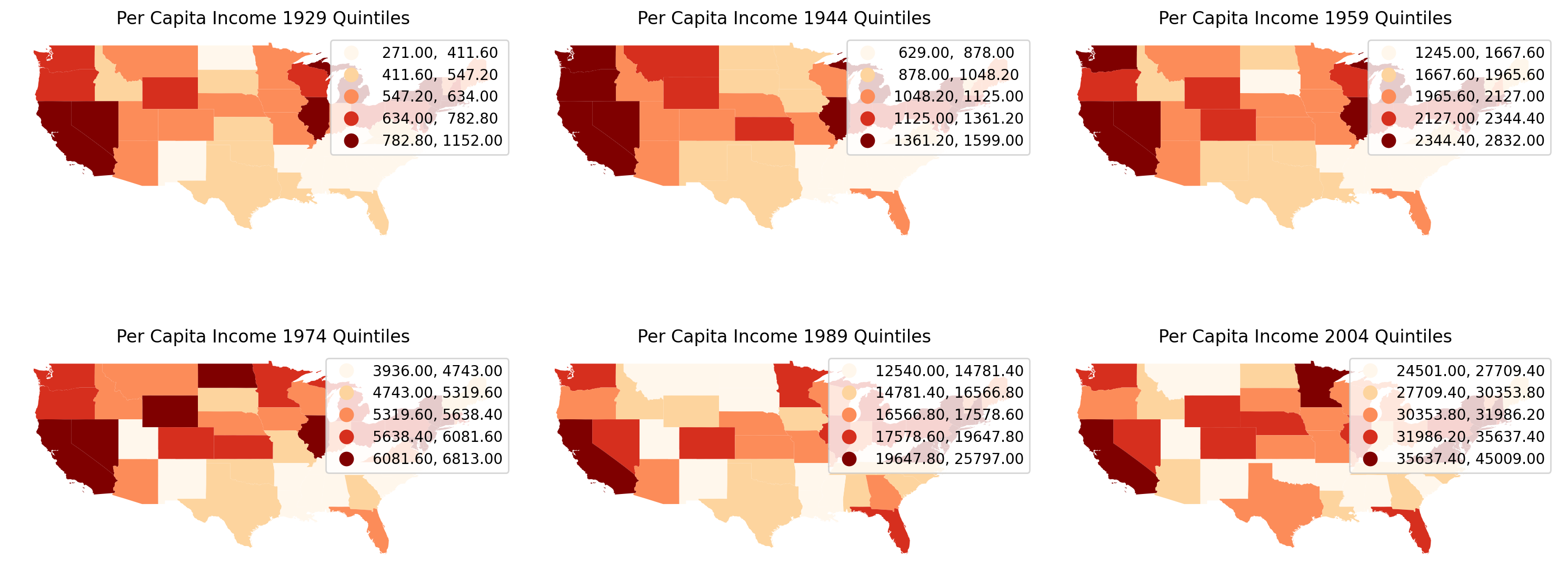
We will visualize the spatial distributions of per capita incomes of US states across 1929 to 2009 to obtain a first impression of the dynamics.

[3]:

import matplotlib.pyplot as plt
import warnings

with warnings.catch_warnings():
    warnings.simplefilter("ignore")
    # ignore geopandas/plotting.py:732:
    # FutureWarning: is_categorical_dtype is deprecated and will be removed in a future version.

    index_year = range(1929, 2010, 15)
    fig, axes = plt.subplots(nrows=2, ncols=3, figsize=(15, 7))
    for i in range(2):
        for j in range(3):
            ax = axes[i, j]
            complete_table.plot(
                ax=ax,
                column=str(index_year[i * 3 + j]),
                cmap="OrRd",
                scheme="quantiles",
                legend=True,
            )
            ax.set_title(f"Per Capita Income {index_year[i*3+j]} Quintiles")
            ax.axis("off")
    plt.tight_layout()

../_images/notebooks_RankBasedMethods_4_0.png

[4]:

years = range(1929, 2010)
names = income_table["Name"]
pci = income_table.drop(columns=["Name", "STATE_FIPS"]).values.T
rpci = (pci.T / pci.mean(axis=1)).T
order1929 = np.argsort(rpci[0, :])
order2009 = np.argsort(rpci[-1, :])
names1929 = names[order1929[::-1]]
names2009 = names[order2009[::-1]]
first_last = np.vstack((names1929, names2009))
from pylab import rcParams

rcParams["figure.figsize"] = 15, 10
p = plt.plot(years, rpci)
for i in range(48):
    plt.text(1915, 1.91 - (i * 0.041), first_last[0][i], fontsize=12)
    plt.text(2010.5, 1.91 - (i * 0.041), first_last[1][i], fontsize=12)
plt.xlim((years[0], years[-1]))
plt.ylim((0, 1.94))
plt.ylabel(r"$y_{i,t}/\bar{y}_t$", fontsize=14)
plt.xlabel("Years", fontsize=12)
plt.title("Relative per capita incomes of 48 US states", fontsize=18)

[4]:

Text(0.5, 1.0, 'Relative per capita incomes of 48 US states')

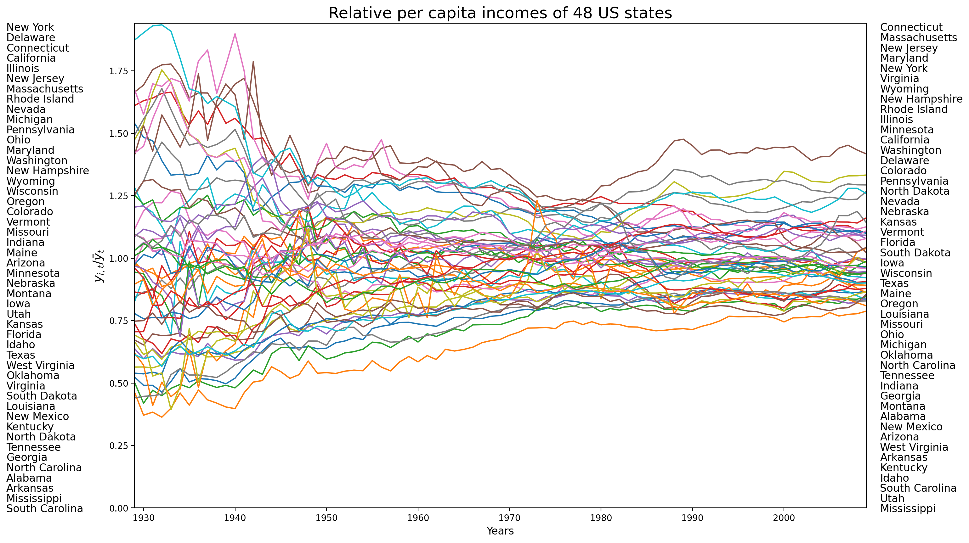
../_images/notebooks_RankBasedMethods_5_1.png

The above figure displays the trajectories of relative per capita incomes of 48 US states. It is quite obvious that states were swapping positions across 1929-2009. We will demonstrate how to quantify the exchange mobility as well as how to assess the regional and local contribution to the overall exchange mobility. We will ultilize BEA regions and base on it for constructing the block weight matrix.

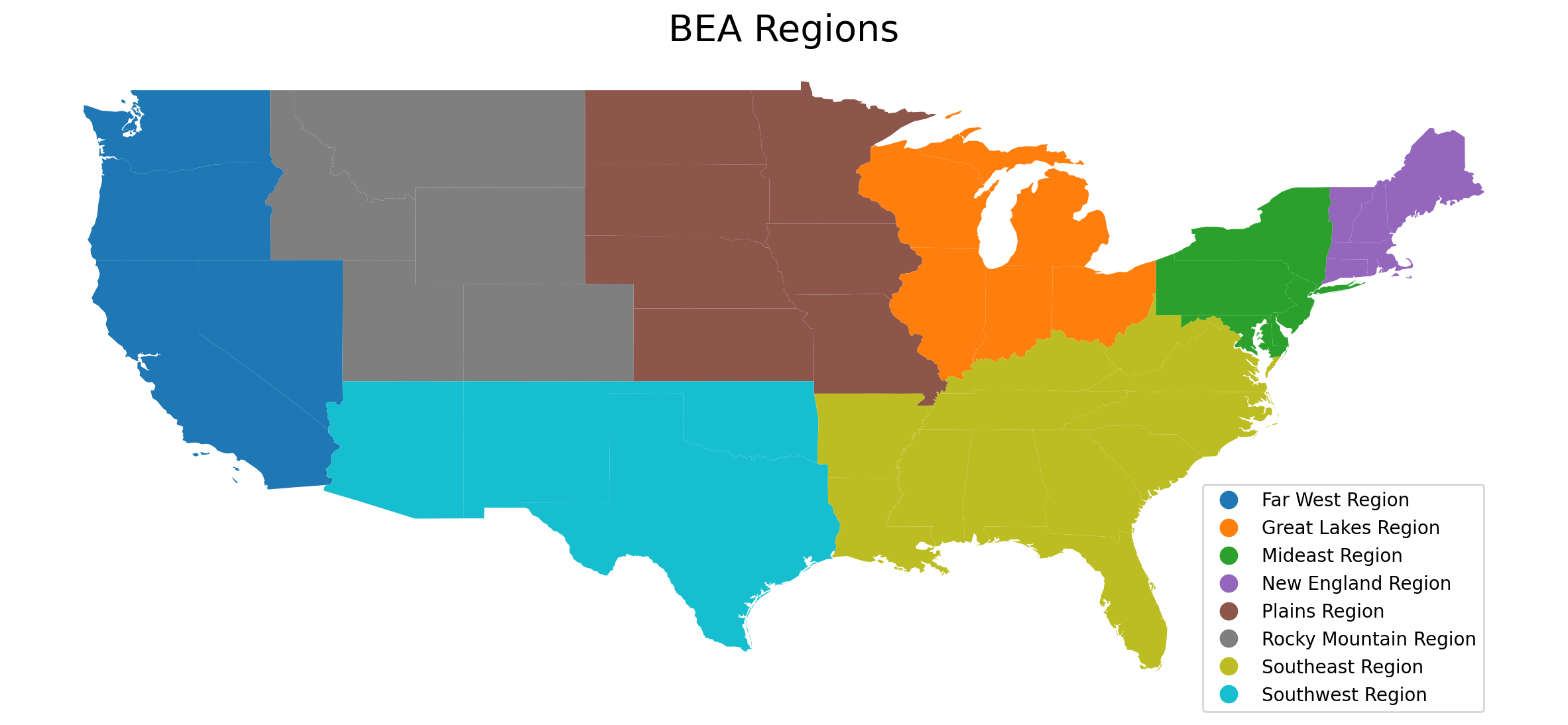
BEA regional scheme divide US states into 8 regions: * New England Region * Mideast Region * Great Lakes Region * Plains Region * Southeast Region * Southwest Region * Rocky Mountain Region * Far West Region

As the dataset does not contain information regarding BEA regions, we manually input the regional information:

[5]:

BEA_regions = [
    "New England Region",
    "Mideast Region",
    "Great Lakes Region",
    "Plains Region",
    "Southeast Region",
    "Southwest Region",
    "Rocky Mountain Region",
    "Far West Region",
]
BEA_regions_abbr = ["NENG", "MEST", "GLAK", "PLNS", "SEST", "SWST", "RKMT", "FWST"]
BEA = pd.DataFrame(
    {
        "Region code": np.arange(1, 9, 1),
        "BEA region": BEA_regions,
        "BEA abbr": BEA_regions_abbr,
    }
)
BEA

[5]:

	Region code	BEA region	BEA abbr
0	1	New England Region	NENG
1	2	Mideast Region	MEST
2	3	Great Lakes Region	GLAK
3	4	Plains Region	PLNS
4	5	Southeast Region	SEST
5	6	Southwest Region	SWST
6	7	Rocky Mountain Region	RKMT
7	8	Far West Region	FWST

[6]:

region_code = (
    list(np.repeat(1, 6))
    + list(np.repeat(2, 6))
    + list(np.repeat(3, 5))
    + list(np.repeat(4, 7))
    + list(np.repeat(5, 12))
    + list(np.repeat(6, 4))
    + list(np.repeat(7, 5))
    + list(np.repeat(8, 6))
)
state_code = (
    ["09", "23", "25", "33", "44", "50", "10", "11", "24", "34", "36", "42", "17"]
    + ["18", "26", "39", "55", "19", "20", "27", "29", "31", "38", "46", "01", "05"]
    + ["12", "13", "21", "22", "28", "37", "45", "47", "51", "54", "04", "35", "40"]
    + ["48", "08", "16", "30", "49", "56", "02", "06", "15", "32", "41", "53"]
)
state_region = pd.DataFrame({"Region code": region_code, "State code": state_code})
state_region_all = state_region.merge(
    BEA, left_on="Region code", right_on="Region code"
)
complete_table = complete_table.merge(
    state_region_all, left_on="STATE_FIPS_x", right_on="State code"
)
complete_table.head()

[6]:

	AREA	PERIMETER	STATE_	STATE_ID	STATE_NAME	STATE_FIPS_x	SUB_REGION	STATE_ABBR	geometry	Name	...	2004	2005	2006	2007	2008	2009	Region code	State code	BEA region	BEA abbr
0	20.750	34.956	1	1	Washington	53	Pacific	WA	MULTIPOLYGON (((-122.40075 48.22540, -122.4615...	Washington	...	34984	35738	38477	40782	41588	40619	8	53	Far West Region	FWST
1	45.132	34.527	2	2	Montana	30	Mtn	MT	POLYGON ((-111.47463 44.70224, -111.48001 44.6...	Montana	...	27517	28987	30942	32625	33293	32699	7	30	Rocky Mountain Region	RKMT
2	9.571	18.899	3	3	Maine	23	N Eng	ME	MULTIPOLYGON (((-69.77779 44.07407, -69.86044 ...	Maine	...	30201	30721	32340	33620	34906	35268	1	23	New England Region	NENG
3	21.874	21.353	4	4	North Dakota	38	W N Cen	ND	POLYGON ((-98.73006 45.93830, -99.00645 45.939...	North Dakota	...	29676	31644	32856	35882	39009	38672	4	38	Plains Region	PLNS
4	22.598	22.746	5	5	South Dakota	46	W N Cen	SD	POLYGON ((-102.78793 42.99532, -103.00541 42.9...	South Dakota	...	31765	32726	33320	35998	38188	36499	4	46	Plains Region	PLNS

5 rows × 96 columns

The BEA regions are visualized below:

[7]:

with warnings.catch_warnings():
    warnings.simplefilter("ignore")
    # ignore geopandas/plotting.py:732:
    # FutureWarning: is_categorical_dtype is deprecated and will be removed in a future version.

    fig, ax = plt.subplots(nrows=1, ncols=1, figsize=(15, 8))
    beaplot = complete_table.plot(ax=ax, column="BEA region", legend=True)
    leg = ax.get_legend()
    leg.set_bbox_to_anchor((0.8, 0.15, 0.16, 0.2))
    beaplot.set_title("BEA Regions", fontdict={"fontsize": 20})
    ax.set_axis_off()

../_images/notebooks_RankBasedMethods_10_0.png

Kendall’s Tau¶

Kendall’s $\tau$ statistic is based on a comparison of the number of pairs of $n$ observations that have concordant ranks between two variables. For measuring exchange mobility in giddy, the two variables in question are the values of an attribute measured at two points in time over $n$ spatial units. This classic measure of rank correlation indicates how much relative stability there has been in the map pattern over the two periods. Spatial decomposition of Kendall’s $\tau$ could be classified into three spatial scales: global spatial decomposition , inter- and intra-regional decomposition and local spatial decomposition. More details will be given latter.

Classic Kendall Tau¶

Kendall’s $\tau$ statistic is a global measure of exchange mobility. For $n$ spatial units over two periods, it is formally defined as follows:

\begin{equation} \tau = \frac{c-d}{(n(n-1))/2} \end{equation}

where $c$ is the number of concordant pairs (two spatial units which do not exchange ranks over two periods), and $d$ is the number of discordant pairs (two spatial units which exchange ranks over two periods). $-1 \leq \tau \leq 1$. Smaller $\tau$ indicates higher exchange mobility.

In giddy, class $Tau$ requires two inputs: a cross-section of income values at one period ($x$) and a cross-section of income values at another period ($y$):

giddy.rank.Tau(self, x, y)

We will construct a $Tau$ instance by specifying the incomes in two periods. Here, we look at the global exchange mobility of US states between 1929 and 2009.

[8]:

with warnings.catch_warnings():
    warnings.simplefilter("ignore")
    # ignore NumbaDeprecationWarning: gh-pysal/libpysal#560

    import giddy

[9]:

tau = giddy.rank.Tau(complete_table["1929"], complete_table["2009"])
tau

[9]:

<giddy.rank.Tau at 0x16fb98310>

[10]:

tau.concordant

[10]:

856.0

[11]:

tau.discordant

[11]:

271.0

There are 856 concordant pairs of US states between 1929 and 2009, and 271 discordant pairs.

[12]:

tau.tau

[12]:

0.5188470576690462

[13]:

tau.tau_p

[13]:

1.9735720263920198e-07

The observed Kendall’s $\tau$ statistic is 0.519 and its p-value is $1.974 \times 10^{-7}$. Therefore, we will reject the null hypothesis of no assocation between 1929 and 2009 at the $5\%$ significance level.

Spatial Kendall Tau¶

The spatial Kendall’s $\tau$ decomposes all pairs into those that are spatial neighbors and those that are not, and examines whether the rank correlation is different between the two sets (Rey, 2014).

\begin{equation} \tau_w = \frac{\iota'(W\circ S)\iota}{\iota'W \iota} \end{equation}

$W$ is the spatial weight matrix, $S$ is the concordance matrix and $\iota$ is the $(n,1)$ unity vector. The null hypothesis is the spatial randomness of rank exchanges. The inference of $\tau_w$ could be conducted based on random spatial permutation of incomes at two periods.

giddy.rank.SpatialTau(self, x, y, w, permutations=0)

For illustration, we turn back to the case of incomes in US states over 1929-2009:

[14]:

from libpysal.weights import block_weights

with warnings.catch_warnings():
    warnings.filterwarnings(
        "ignore", message="The weights matrix is not fully connected"
    )

    w = block_weights(complete_table["BEA region"])
    np.random.seed(12345)
    tau_w = giddy.rank.SpatialTau(
        complete_table["1929"], complete_table["2009"], w, 999
    )

[15]:

tau_w.concordant

[15]:

856.0

[16]:

tau_w.concordant_spatial

[16]:

[17]:

tau_w.discordant

[17]:

271.0

[18]:

tau_w.discordant_spatial

[18]:

Out of 856 concordant pairs of spatial units, 103 belong to the same region (and are considered neighbors); out of 271 discordant pairs of spatial units, 41 belong to the same region.

[19]:

tau_w.tau_spatial

[19]:

0.4305555555555556

[20]:

tau_w.tau_spatial_psim

[20]:

0.001

The estimate of spatial Kendall’s $\tau$ is 0.431 and its p-value is 0.001 which is much smaller than the significance level $0.05$. Therefore, we reject the null of spatial randomness of exchange mobility. The fact that tau_w=0.431 is smaller than the global average $\tau=0.519$ implies that globally a significant number of rank exchanges happened between states within the same region though we do not know the specific region or regions hosting these rank exchanges. A more thorough decomposition of $\tau$ such as inter- and intra-regional indicators and local indicators will provide insights on this issue.

Inter- and Intra-regional decomposition of Kendall’s Tau¶

A meso-level view on the exchange mobility pattern is provided by inter- and intra-regional decomposition of Kendall’s $\tau$. This decomposition can shed light on specific regions hosting most rank exchanges. More precisely, insteading of examining the concordance relationship between any two neighboring spatial units in the whole study area, for a specific region A, we examine the concordance relationship between any two spatial units within region A (neighbors), resulting in the intraregional concordance statistic for A; or we could examine the concordance relationship between any spatial unit in region A and any spatial unit in region B (nonneighbors), resulting in the interregional concordance statistic for A and B. If there are k regions, there will be k intraregional concordance statistics and $(k-1)^2$ interregional concordance statistics, we could organize them into a $(k,k)$ matrix where the diagonal elements are intraregional concordance statistics and nondiagnoal elements are interregional concordance statistics.

Formally, this inter- and intra-regional concordance statistic matrix is defined as follows (Rey, 2016):

\begin{equation} T=\frac{P(H \circ S)P'}{P H P'} \end{equation}

$P$ is a $(k,n)$ binary matrix where $p_{j,i}=1$ if spatial unit $i$ is in region $j$ and $p_{j,i}=0$ otherwise. $H$ is a $(n,n)$ matrix with 0 on diagnoal and 1 on other places. $\circ$ is the Hadamard product. Inference could be based on random spatial permutation of incomes at two periods, similar to spatial $\tau$.

To obtain an estimate for the inter- and intra-regional indicator matrix, we use the Tau_Regional class:

giddy.rank.Tau_Regional(self, x, y, regime, permutations=0)

Here, regime is an 1-dimensional array of size n. Each element is the id of which region an spatial unit belongs to.

[21]:

?giddy.rank.Tau_Regional

Init signature: giddy.rank.Tau_Regional(x, y, regime, permutations=0)
Docstring:
Inter and intraregional decomposition of the classic Tau.

Parameters
----------
x               : array
                  (n, ), first variable.
y               : array
                  (n, ), second variable.
regimes         : array
                  (n, ), ids of which regime an observation belongs to.
permutations    : int
                  number of random spatial permutations for
                  computationally based inference.

Attributes
----------
n               : int
                  number of observations.
S               : array
                  (n ,n), concordance matrix, s_{i,j}=1 if
                  observation i and j are concordant, s_{i,
                  j}=-1 if observation i and j are discordant,
                  and s_{i,j}=0 otherwise.
tau_reg         : array
                  (k, k), observed concordance matrix with
                  diagonal elements measuring concordance
                  between units within a regime and the
                  off-diagonal elements denoting concordance
                  between observations from a specific
                  pair of different regimes.
tau_reg_sim     : array
                  (permutations, k, k), concordance matrices for
                  permuted samples (if permutations>0).
tau_reg_pvalues : array
                  (k, k), one-sided pseudo p-values for observed
                  concordance matrix under the null that income
                  mobility were random in its spatial distribution.

Notes
-----
The equation for calculating inter and intraregional Tau
statistic can be found in :cite:`Rey2016` Equation (27).

Examples
--------
>>> import libpysal as ps
>>> import numpy as np
>>> from giddy.rank import Tau_Regional
>>> np.random.seed(10)
>>> f = ps.io.open(ps.examples.get_path("mexico.csv"))
>>> vnames = ["pcgdp%d"%dec for dec in range(1940, 2010, 10)]
>>> y = np.transpose(np.array([f.by_col[v] for v in vnames]))
>>> r = y / y.mean(axis=0)
>>> regime = np.array(f.by_col['esquivel99'])
>>> res = Tau_Regional(y[:,0],y[:,-1],regime,permutations=999)
>>> res.tau_reg
array([[1.        , 0.25      , 0.5       , 0.6       , 0.83333333,
        0.6       , 1.        ],
       [0.25      , 0.33333333, 0.5       , 0.3       , 0.91666667,
        0.4       , 0.75      ],
       [0.5       , 0.5       , 0.6       , 0.4       , 0.38888889,
        0.53333333, 0.83333333],
       [0.6       , 0.3       , 0.4       , 0.2       , 0.4       ,
        0.28      , 0.8       ],
       [0.83333333, 0.91666667, 0.38888889, 0.4       , 0.6       ,
        0.73333333, 1.        ],
       [0.6       , 0.4       , 0.53333333, 0.28      , 0.73333333,
        0.8       , 0.8       ],
       [1.        , 0.75      , 0.83333333, 0.8       , 1.        ,
        0.8       , 0.33333333]])
>>> res.tau_reg_pvalues
array([[0.782, 0.227, 0.464, 0.638, 0.294, 0.627, 0.201],
       [0.227, 0.352, 0.391, 0.14 , 0.048, 0.252, 0.327],
       [0.464, 0.391, 0.587, 0.198, 0.107, 0.423, 0.124],
       [0.638, 0.14 , 0.198, 0.141, 0.184, 0.089, 0.217],
       [0.294, 0.048, 0.107, 0.184, 0.583, 0.25 , 0.005],
       [0.627, 0.252, 0.423, 0.089, 0.25 , 0.38 , 0.227],
       [0.201, 0.327, 0.124, 0.217, 0.005, 0.227, 0.322]])
File:           ~/giddy/giddy/rank.py
Type:           type
Subclasses:

Similar to before, we go back to the case of incomes in US states over 1929-2009:

[22]:

with warnings.catch_warnings():
    warnings.filterwarnings(
        "ignore", message="The weights matrix is not fully connected"
    )
    np.random.seed(12345)

    tau_w = giddy.rank.Tau_Regional(
        complete_table["1929"],
        complete_table["2009"],
        complete_table["BEA region"],
        999,
    )

[23]:

tau_w.tau_reg

[23]:

array([[ 0.66666667,  0.5       ,  0.3       ,  0.41666667,  0.28571429,
         0.5       ,  0.79166667,  0.875     ],
       [ 0.5       ,  0.4       ,  0.52      ,  0.26666667, -0.48571429,
         0.52      ,  0.53333333,  0.6       ],
       [ 0.3       ,  0.52      ,  0.        ,  0.4       ,  0.88571429,
         0.76      ,  0.93333333,  1.        ],
       [ 0.41666667,  0.26666667,  0.4       ,  0.86666667,  0.47619048,
         0.83333333,  0.86111111,  0.91666667],
       [ 0.28571429, -0.48571429,  0.88571429,  0.47619048, -0.14285714,
         0.42857143,  0.69047619,  0.14285714],
       [ 0.5       ,  0.52      ,  0.76      ,  0.83333333,  0.42857143,
         0.8       ,  0.06666667,  0.1       ],
       [ 0.79166667,  0.53333333,  0.93333333,  0.86111111,  0.69047619,
         0.06666667,  0.54545455,  0.33333333],
       [ 0.875     ,  0.6       ,  1.        ,  0.91666667,  0.14285714,
         0.1       ,  0.33333333,  0.        ]])

The attribute tau_reg gives the inter- and intra-regional concordance statistic matrix. Higher values represents lower exchange mobility. Obviously there are some negative values indicating high exchange mobility. Attribute tau_reg_pvalues gives pvalues for all inter- and intra-regional concordance statistics:

[24]:

tau_w.tau_reg_pvalues

[24]:

array([[0.586, 0.516, 0.196, 0.37 , 0.151, 0.526, 0.051, 0.104],
       [0.516, 0.41 , 0.583, 0.114, 0.001, 0.532, 0.526, 0.472],
       [0.196, 0.583, 0.102, 0.316, 0.011, 0.156, 0.001, 0.014],
       [0.37 , 0.114, 0.316, 0.122, 0.41 , 0.034, 0.003, 0.026],
       [0.151, 0.001, 0.011, 0.41 , 0.013, 0.344, 0.08 , 0.051],
       [0.526, 0.532, 0.156, 0.034, 0.344, 0.324, 0.005, 0.056],
       [0.051, 0.526, 0.001, 0.003, 0.08 , 0.005, 0.502, 0.136],
       [0.104, 0.472, 0.014, 0.026, 0.051, 0.056, 0.136, 0.166]])

We can manipulate these two attribute to obtain significant inter- and intra-regional statistics only (at the $5\%$ significance level):

[25]:

tau_w.tau_reg * (tau_w.tau_reg_pvalues < 0.05)

[25]:

array([[ 0.        ,  0.        ,  0.        ,  0.        ,  0.        ,
         0.        ,  0.        ,  0.        ],
       [ 0.        ,  0.        ,  0.        ,  0.        , -0.48571429,
         0.        ,  0.        ,  0.        ],
       [ 0.        ,  0.        ,  0.        ,  0.        ,  0.88571429,
         0.        ,  0.93333333,  1.        ],
       [ 0.        ,  0.        ,  0.        ,  0.        ,  0.        ,
         0.83333333,  0.86111111,  0.91666667],
       [ 0.        , -0.48571429,  0.88571429,  0.        , -0.14285714,
         0.        ,  0.        ,  0.        ],
       [ 0.        ,  0.        ,  0.        ,  0.83333333,  0.        ,
         0.        ,  0.06666667,  0.        ],
       [ 0.        ,  0.        ,  0.93333333,  0.86111111,  0.        ,
         0.06666667,  0.        ,  0.        ],
       [ 0.        ,  0.        ,  1.        ,  0.91666667,  0.        ,
         0.        ,  0.        ,  0.        ]])

The table below displays the inter- and intra-regional decomposition matrix of Kendall’s $\tau$ for US states over 1929-2009 based on the 8 BEA regions. Bold numbers indicate significance at the $5\%$ significance level. The negative and significant intra-Southeast concordance statistic ($-0.486$) indicates that the rank exchanges within Southeast region is significantly more frequent than those between states within and out of Southeast region.

Region	New England	Mideast	Great Lakes	Plains	Southeast	Southwest	Rocky Mountain	Far West
New England	0.667	0.5	0.3	0.417	0.2856	0.5	0.792	0.875
Mideast	0.5	0.4	0.52	0.267	-0.486	0.52	0.533	0.6
Great Lakes	0.3	0.52	0	0.4	0.886	0.76	0.933
Plains	0.417	0.267	0.4	0.867	0.476	0.833	0.861	0.917
Southeast	0.286	-0.486	0.886	0.476	-0.143	0.429	0.690	0.143
Southwest	0.5	0.52	0.76	0.833	0.429	0.8	0.067	0.1
Rocky Mountain	0.792	0.533	0.933	0.861	0.69	0.067	0.545	0.333
Far West	0.875	0.6		0.917	0.143	0.1	0.333	0

Local Kendall Tau¶

Local Kendall’s $\tau$ is a local decomposition of classic Kendall’s $\tau$ which provides an indication of the contribution of spatial unit $r$’s rank changes to the overall level of exchange mobility (Rey, 2016). Focusing on spatial unit $r$, we formally define it as follows:

\begin{equation} \tau_{r} = \frac{c_r - d_r}{n-1} \end{equation}

where $c_r$ is the number of spatial units (except $r$) which are concordant with $r$ and $d_r$ is the number of spatial units which are discordant with $r$. Similar to classic Kendall’s $\tau$, local $\tau$ takes values on $[-1,1]$. The larger the value, the lower the exchange mobility for $r$.

giddy.rank.Tau_Local(self, x, y)

We create a Tau_Local instance for US dynamics 1929-2009:

[26]:

tau_r = giddy.rank.Tau_Local(complete_table["1929"], complete_table["2009"])
tau_r

[26]:

<giddy.rank.Tau_Local at 0x1703bab10>

[27]:

pd.DataFrame(
    {"STATE_NAME": complete_table["STATE_NAME"].tolist(), "$\\tau_r$": tau_r.tau_local}
).head()

[27]:

	STATE_NAME	$\tau_r$
0	Washington	0.617021
1	Montana	0.446809
2	Maine	0.404255
3	North Dakota	-0.021277
4	South Dakota	0.319149

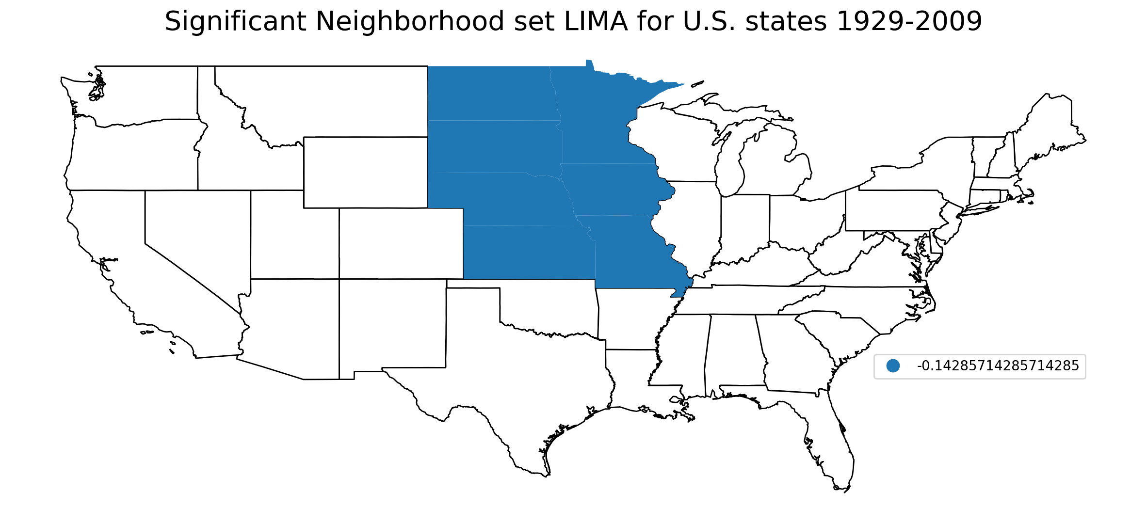
Therefore, local concordance measure produces a negative value for North Dakota (-0.0213) indicating that North Dakota exchanged ranks with a lot of states across 1929-2000. On the contrary, the local $\tau$ statistic is quite high for Washington (0.617) highlighting a high stability of Washington.

Local indicator of mobility association-LIMA¶

To reveal the role of space in shaping the exchange mobility pattern for each spatial unit, two spatial variants of local Kendall’s $\tau$ could be utilized: neighbor set LIMA and neighborhood set LIMA (Rey, 2016). The latter is also the result of a decomposition of local Kendall’s $\tau$ (into neighboring and nonneighboring parts) as well as a decompostion of spatial Kendall’s $\tau$ (into its local components).

Neighbor set LIMA¶

Instead of examining the concordance relationship between a focal spatial unit $r$ and all the other units as what local $\tau$ does, neighbor set LIMA focuses on the concordance relationship between a focal spatial unit $r$ and its neighbors only. It is formally defined as follows:

\begin{equation} \tilde{\tau}_{r} = \frac{\sum_b w_{r,b} s_{r,b}}{\sum_b w_{r,b}} \end{equation}

giddy.rank.Tau_Local_Neighbor(self, x, y, w, permutations=0)

[28]:

tau_wr = giddy.rank.Tau_Local_Neighbor(
    complete_table["1929"], complete_table["2009"], w, 999
)
tau_wr

[28]:

<giddy.rank.Tau_Local_Neighbor at 0x16faf0a50>

[29]:

tau_wr.tau_ln

[29]:

array([ 0.33333333,  1.        ,  1.        , -0.66666667,  0.        ,
        1.        ,  0.        ,  0.5       ,  1.        ,  0.66666667,
        1.        ,  0.6       , -0.33333333,  1.        ,  0.33333333,
        0.        ,  0.5       ,  1.        ,  0.6       ,  0.        ,
        1.        ,  0.33333333,  0.5       ,  1.        ,  0.        ,
        1.        ,  0.        , -0.09090909, -0.5       ,  1.        ,
        0.09090909,  0.        ,  0.63636364, -1.        , -1.        ,
        0.33333333,  0.27272727,  0.45454545,  0.33333333,  0.33333333,
        0.63636364,  0.81818182,  0.45454545,  0.81818182,  0.81818182,
        0.81818182,  0.81818182,  0.        ])

To visualize the spatial distribution of neighbor set LIMA:

[30]:

with warnings.catch_warnings():
    warnings.simplefilter("ignore")
    # ignore geopandas/plotting.py:732:
    # FutureWarning: is_categorical_dtype is deprecated and will be removed in a future version.

    complete_table["tau_ln"] = tau_wr.tau_ln
    fig, ax = plt.subplots(nrows=1, ncols=1, figsize=(15, 8))
    ln_map = complete_table.plot(
        ax=ax, column="tau_ln", cmap="coolwarm", scheme="equal_interval", legend=True
    )
    leg = ax.get_legend()
    leg.set_bbox_to_anchor((0.8, 0.15, 0.16, 0.2))
    ln_map.set_title(
        "Neighbor set LIMA for U.S. states 1929-2009", fontdict={"fontsize": 20}
    )
    ax.set_axis_off()

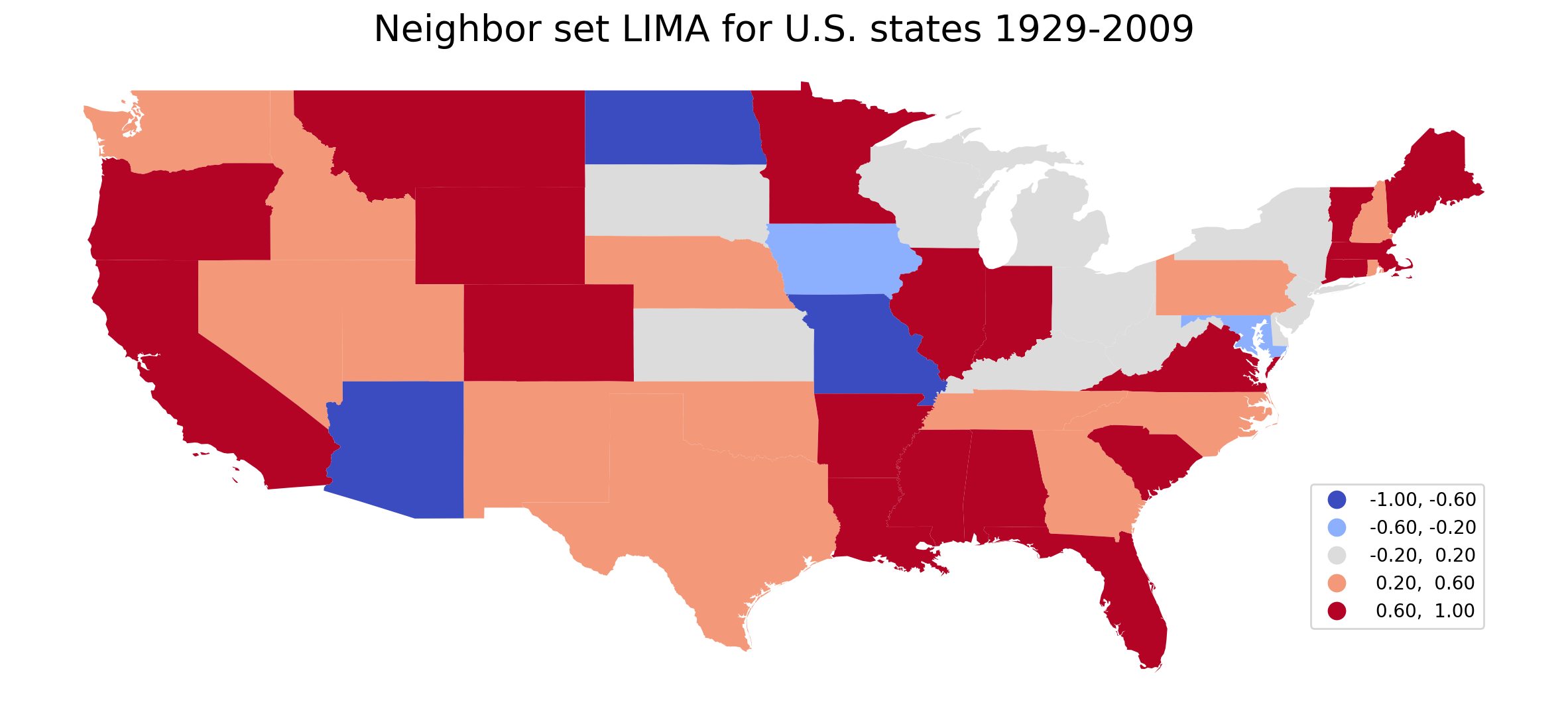
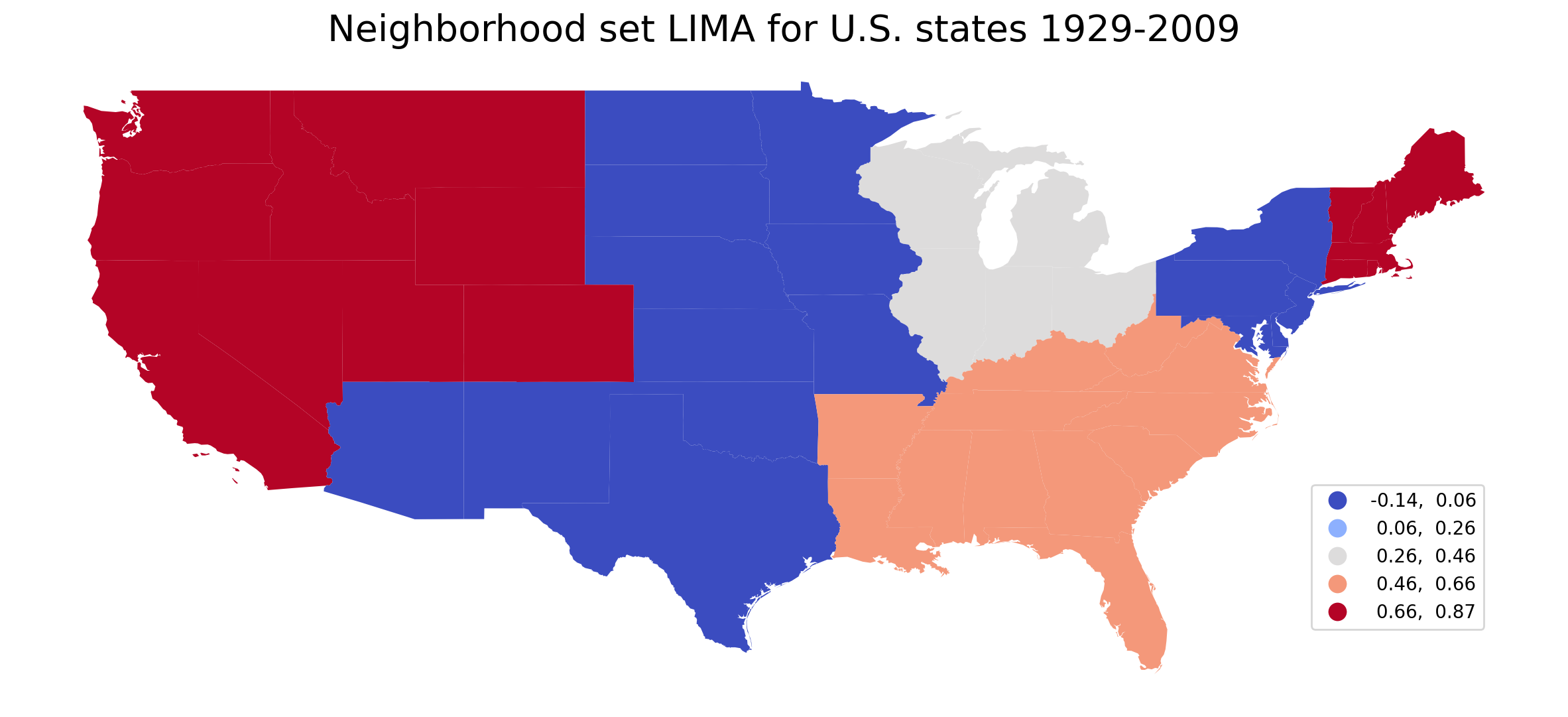
../_images/notebooks_RankBasedMethods_46_0.png

Therefore, Arizona, North Dakota, and Missouri exchanged ranks with most of their neighbors over 1929-2009 while California, Virginia etc. barely exchanged ranks with their neighbors.

Let see whether neighbor set LIMA statistics are siginificant for these “extreme” states:

[31]:

tau_wr.tau_ln_pvalues

[31]:

array([0.463, 0.256, 0.165, 0.101, 0.316, 0.336, 0.237, 0.614, 0.292,
       0.325, 0.33 , 0.675, 0.06 , 0.541, 0.412, 0.032, 0.594, 0.791,
       0.575, 0.049, 0.209, 0.48 , 0.488, 0.457, 0.605, 0.409, 0.259,
       0.018, 0.022, 0.405, 0.016, 0.25 , 0.001, 0.001, 0.045, 0.521,
       0.167, 0.363, 0.635, 0.478, 0.417, 0.247, 0.282, 0.423, 0.578,
       0.17 , 0.1  , 0.625])

[32]:

sig_wr = tau_wr.tau_ln * (tau_wr.tau_ln_pvalues < 0.05)
sig_wr

[32]:

array([ 0.        ,  0.        ,  0.        , -0.        ,  0.        ,
        0.        ,  0.        ,  0.        ,  0.        ,  0.        ,
        0.        ,  0.        , -0.        ,  0.        ,  0.        ,
        0.        ,  0.        ,  0.        ,  0.        ,  0.        ,
        0.        ,  0.        ,  0.        ,  0.        ,  0.        ,
        0.        ,  0.        , -0.09090909, -0.5       ,  0.        ,
        0.09090909,  0.        ,  0.63636364, -1.        , -1.        ,
        0.        ,  0.        ,  0.        ,  0.        ,  0.        ,
        0.        ,  0.        ,  0.        ,  0.        ,  0.        ,
        0.        ,  0.        ,  0.        ])

[33]:

with warnings.catch_warnings():
    warnings.simplefilter("ignore")
    # ignore geopandas/plotting.py:732:
    # FutureWarning: is_categorical_dtype is deprecated and will be removed in a future version.

    complete_table["sig_wr"] = sig_wr
    fig, ax = plt.subplots(nrows=1, ncols=1, figsize=(15, 8))
    complete_table[complete_table["sig_wr"] == 0].plot(
        ax=ax, color="white", edgecolor="black"
    )
    sig_ln_map = complete_table[complete_table["sig_wr"] != 0].plot(
        ax=ax, column="sig_wr", cmap="coolwarm", scheme="equal_interval", legend=True
    )
    leg = ax.get_legend()
    leg.set_bbox_to_anchor((0.8, 0.15, 0.16, 0.2))
    sig_ln_map.set_title(
        "Significant Neighbor set LIMA for U.S. states 1929-2009",
        fontdict={"fontsize": 20},
    )
    ax.set_axis_off()

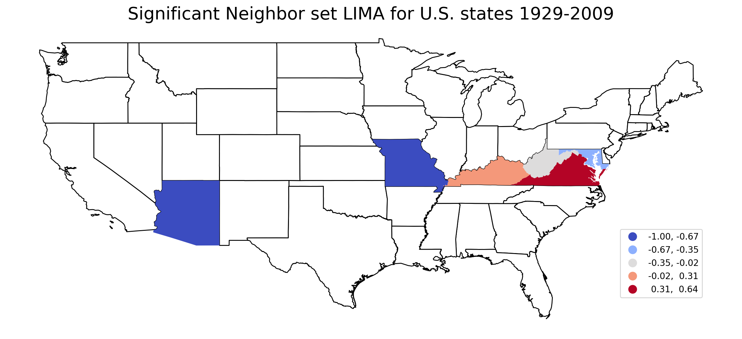
../_images/notebooks_RankBasedMethods_50_0.png

Thus, Arizona and Missouri have significant and negative neighbor set LIMA values, and can be considered as hotspots of rank exchanges. This means that Arizona (or Missouri) tended to exchange ranks with its neighbors than with others over 1929-2009. On the contrary, Virgina has significant and large positive neighbor set LIMA value indicating that it tended to exchange ranks with its nonneighbors than with neighbors.

Neighborhood set LIMA¶

Neighborhood set LIMA extends neighbor set LIMA $\tilde{\tau}_{r}$ to consider the concordance relationships between any two spatial units in the subset which is composed of the focal unit $r$ and its neighbors.

giddy.rank.Tau_Local_Neighborhood(self, x, y, w, permutations=0)

[34]:

tau_wwr = giddy.rank.Tau_Local_Neighborhood(
    complete_table["1929"], complete_table["2009"], w, 999
)
tau_wwr

[34]:

<giddy.rank.Tau_Local_Neighborhood at 0x1703c9bd0>

[35]:

tau_wwr.tau_lnhood

[35]:

array([ 0.66666667,  0.8       ,  0.86666667, -0.14285714, -0.14285714,
        0.8       ,  0.4       ,  0.8       ,  0.86666667, -0.14285714,
        0.66666667,  0.86666667, -0.14285714,  0.86666667, -0.14285714,
        0.        ,  0.        ,  0.86666667,  0.86666667,  0.        ,
        0.4       ,  0.66666667,  0.8       ,  0.66666667,  0.4       ,
        0.4       ,  0.        ,  0.54545455,  0.        ,  0.8       ,
        0.54545455, -0.14285714,  0.54545455, -0.14285714,  0.        ,
        0.        ,  0.54545455,  0.54545455,  0.        ,  0.        ,
        0.54545455,  0.54545455,  0.54545455,  0.54545455,  0.54545455,
        0.54545455,  0.54545455,  0.4       ])

[36]:

with warnings.catch_warnings():
    warnings.simplefilter("ignore")
    # ignore geopandas/plotting.py:732:
    # FutureWarning: is_categorical_dtype is deprecated and will be removed in a future version.

    complete_table["tau_lnhood"] = tau_wwr.tau_lnhood
    fig, ax = plt.subplots(nrows=1, ncols=1, figsize=(15, 8))
    ln_map = complete_table.plot(
        ax=ax,
        column="tau_lnhood",
        cmap="coolwarm",
        scheme="equal_interval",
        legend=True,
    )
    leg = ax.get_legend()
    leg.set_bbox_to_anchor((0.8, 0.15, 0.16, 0.2))
    ln_map.set_title(
        "Neighborhood set LIMA for U.S. states 1929-2009", fontdict={"fontsize": 20}
    )
    ax.set_axis_off()

../_images/notebooks_RankBasedMethods_54_0.png

[37]:

tau_wwr.tau_lnhood_pvalues

[37]:

array([0.585, 0.278, 0.104, 0.032, 0.024, 0.295, 0.43 , 0.225, 0.167,
       0.02 , 0.548, 0.116, 0.023, 0.158, 0.017, 0.016, 0.075, 0.225,
       0.168, 0.027, 0.505, 0.66 , 0.146, 0.605, 0.614, 0.37 , 0.08 ,
       0.505, 0.059, 0.358, 0.541, 0.025, 0.185, 0.017, 0.225, 0.151,
       0.541, 0.527, 0.191, 0.12 , 0.519, 0.427, 0.526, 0.442, 0.453,
       0.528, 0.478, 0.617])

[38]:

sig_lnhood = tau_wwr.tau_lnhood * (tau_wwr.tau_lnhood_pvalues < 0.05)
sig_lnhood

[38]:

array([ 0.        ,  0.        ,  0.        , -0.14285714, -0.14285714,
        0.        ,  0.        ,  0.        ,  0.        , -0.14285714,
        0.        ,  0.        , -0.14285714,  0.        , -0.14285714,
        0.        ,  0.        ,  0.        ,  0.        ,  0.        ,
        0.        ,  0.        ,  0.        ,  0.        ,  0.        ,
        0.        ,  0.        ,  0.        ,  0.        ,  0.        ,
        0.        , -0.14285714,  0.        , -0.14285714,  0.        ,
        0.        ,  0.        ,  0.        ,  0.        ,  0.        ,
        0.        ,  0.        ,  0.        ,  0.        ,  0.        ,
        0.        ,  0.        ,  0.        ])

[39]:

with warnings.catch_warnings():
    warnings.simplefilter("ignore")
    # ignore geopandas/plotting.py:732:
    # FutureWarning: is_categorical_dtype is deprecated and will be removed in a future version.

    complete_table["sig_lnhood"] = sig_lnhood
    fig, ax = plt.subplots(nrows=1, ncols=1, figsize=(15, 8))
    complete_table[complete_table["sig_lnhood"] == 0].plot(
        ax=ax, color="white", edgecolor="black"
    )
    sig_ln_map = complete_table[complete_table["sig_lnhood"] != 0].plot(
        ax=ax, column="sig_lnhood", categorical=True, legend=True
    )
    leg = ax.get_legend()
    leg.set_bbox_to_anchor((0.8, 0.15, 0.16, 0.2))
    sig_ln_map.set_title(
        "Significant Neighborhood set LIMA for U.S. states 1929-2009",
        fontdict={"fontsize": 20},
    )
    ax.set_axis_off()

../_images/notebooks_RankBasedMethods_57_0.png

Theta statistic of exchange mobility¶

Next steps¶

theta statistic

References¶

Rey, Sergio J., and Myrna L. Sastré-Gutiérrez. 2010. “Interregional Inequality Dynamics in Mexico.” Spatial Economic Analysis 5 (3). Taylor & Francis: 277–98.
Rey, Sergio J. 2014. “Fast Algorithms for a Space-Time Concordance Measure.” Computational Statistics 29 (3-4). Springer: 799–811.
Rey, Sergio J. 2016. “Space–Time Patterns of Rank Concordance: Local Indicators of Mobility Association with Application to Spatial Income Inequality Dynamics.” Annals of the Association of American Geographers. Association of American Geographers 106 (4): 788–803.