Global Spatial Autocorrelation with Join Counts
This notebook focuses on global spatial autocorrelation for a binary attribute using Join Counts.
Learning goals
By the end of this notebook, you will be able to:
convert a continuous variable into a binary outcome for categorical spatial analysis
understand what a join count measures on a binary spatial lattice
distinguish BB, WW, and BW joins
use permutation inference to assess whether similar categories cluster in space
Join counts are appropriate when the variable of interest is binary rather than continuous.
import geopandas as gpd
import matplotlib.pyplot as plt
import numpy as np
import scipy.stats as stats
import seaborn as sns
from libpysal import graph

import esda
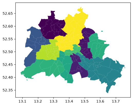
Our data set comes from the Berlin airbnb scrape taken in April 2018. This dataframe was constructed as part of the GeoPython 2018 workshop by Levi Wolf and Serge Rey. As part of the workshop a geopandas data frame was constructed with one of the columns reporting the median listing price of units in each neighborhood in Berlin:
Data preparation
As in the Moran’s \(I\) notebook, we build neighborhood-level median Airbnb prices. We then convert that continuous measure into a binary indicator based on whether a neighborhood is above or below the median price.
df = gpd.read_file("data/berlin-housing.gpkg")
df.plot(column="median_pri")
<Axes: >
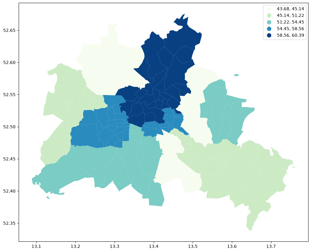
df.plot(
    column="median_pri",
    scheme="Quantiles",
    k=5,
    cmap="GnBu",
    legend=True,
    figsize=(12, 10),
)
<Axes: >
Join Counts
Moran’s \(I\) and Geary’s \(C\) are designed for continuous variables. Once we dichotomize spatial data into binary high and low categories, a different global statistic is more natural: the join count, which evaluates whether like-valued neighbors occur more often than expected by chance.
For a binary map where locations are classified as either Black (\(B\), representing high values or presence) or White (\(W\), representing low values or absence), each neighboring pair of zones forms a “join” mapped via our spatial weights object. Every join falls into one of three mutually exclusive categories:
BB: both neighbors are in the high-value category (Black-Black)
WW: both neighbors are in the low-value category (White-White)
BW: one neighbor is high-value and the other is low-value (Black-White)
Let \(x_i \in \{0, 1\}\) be the binary indicator for location \(i\), where \(x_i = 1\) if the location is Black (\(B\)) and \(x_i = 0\) if the location is White (\(W\)). The count of Black-Black (BB) joins is defined as:
where \(w_{ij}\) is the binary spatial weight expressing the neighbor relationship between locations \(i\) and \(j\). Similarly, White-White (WW) and Black-White (BW) joins are formulated as:
The total number of joins in the network is given by half the sum of the spatial weights matrix elements (\(S_0\)), which completely exhausts all structural possibilities:
Global Join Counts
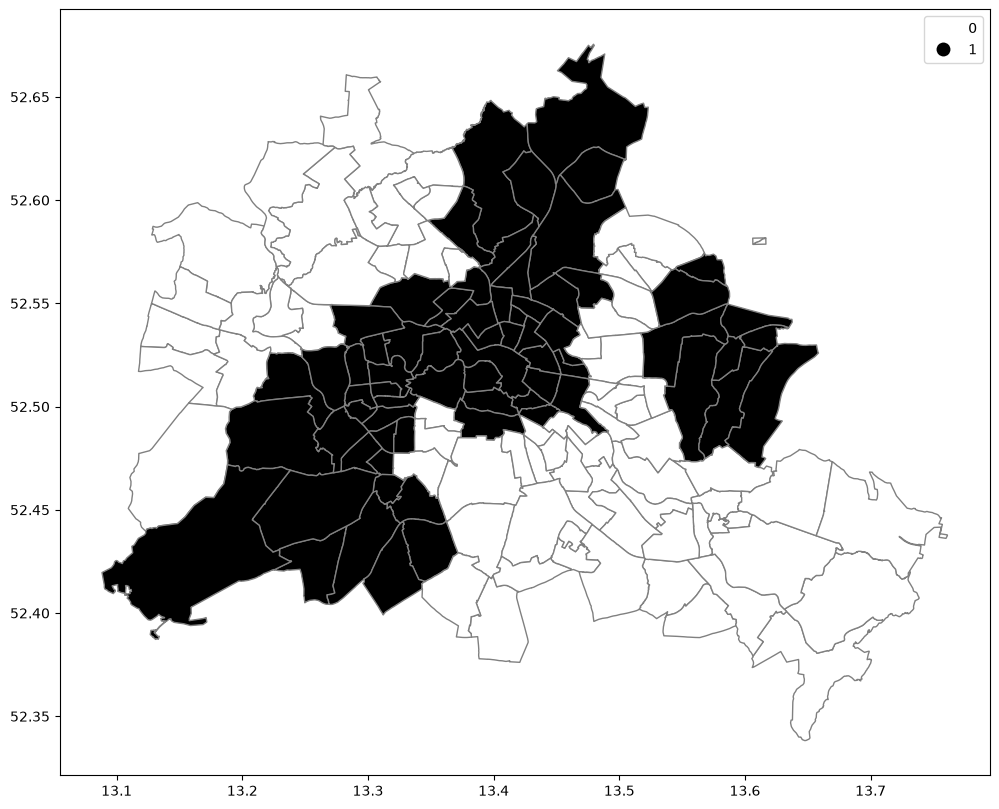
We convert our continuous measure of median Airbnb prices into a binary indicator based on whether a neighborhood sits above or below the median study-wide price. We then construct a binary Queen contiguity matrix to compute the global join count statistics.
df.head()
| neighbourhood | neighbourhood_group | median_pri | yb_binary | geometry | |
|---|---|---|---|---|---|
| 0 | Blankenfelde/Niederschönhausen | Pankow | 60.282516 | 1 | MULTIPOLYGON (((13.41191 52.61487, 13.41183 52... |
| 1 | Helmholtzplatz | Pankow | 60.282516 | 1 | MULTIPOLYGON (((13.41405 52.54929, 13.41422 52... |
| 2 | Wiesbadener Straße | Charlottenburg-Wilm. | 58.556408 | 1 | MULTIPOLYGON (((13.30748 52.46788, 13.30743 52... |
| 3 | Schmöckwitz/Karolinenhof/Rauchfangswerder | Treptow - Köpenick | 51.222004 | 0 | MULTIPOLYGON (((13.70973 52.3963, 13.70926 52.... |
| 4 | Müggelheim | Treptow - Köpenick | 51.222004 | 0 | MULTIPOLYGON (((13.73762 52.4085, 13.73773 52.... |
df.plot(
    column="yb_binary",
    cmap="binary",
    categorical=True,
    edgecolor="grey",
    legend=True,
    figsize=(12, 10),
);
y = df["median_pri"]

yb = 1 * (y > y.median())  # convert to binary
wq = graph.Graph.build_contiguity(df, rook=False)

np.random.seed(12345)
jc = esda.join_counts.Join_Counts(yb, wq)

print(f"Observed BB Joins: {jc.bb}")
print(f"Observed WW Joins: {jc.ww}")
print(f"Observed BW Joins: {jc.bw}")
print(f"Total Joins (K):   {jc.bb + jc.ww + jc.bw}")
Observed BB Joins: 164.0
Observed WW Joins: 149.0
Observed BW Joins: 73.0
Total Joins (K):   386.0
Inference
Inference about join counts evaluates whether the observed number of joins deviates significantly from what we would expect under the null hypothesis of Complete Spatial Randomness (CSR).
To derive the analytical expected values and variances for statistical inference, we define structural constants based on the topology of the weights matrix \(W\):
\(S_0 = \sum_{i=1}^n \sum_{j=1}^n w_{ij}\) (The sum of all spatial weights)
\(S_1 = \frac{1}{2} \sum_{i=1}^n \sum_{j=1}^n (w_{ij} + w_{ji})^2\)
\(S_2 = \sum_{i=1}^n \left( \sum_{j=1}^n w_{ij} + \sum_{j=1}^n w_{ji} \right)^2\)
Let \(B = \sum_{i=1}^n x_i\) be the total count of Black zones, and \(W = n - B\) be the total count of White zones.
Free Sampling (The Normality Assumption)
Under free sampling, it is assumed that each zone has an independent probability \(p = B/n\) of being assigned a Black label, corresponding to sampling with replacement from a population.
Expected Value
The expected number of Black-Black joins depends entirely on the total network joins and the global probability \(p\):
Variance
The analytical variance under free sampling isolates interaction loops using structural constants \(S_1\) and \(S_2\):
Non-Free Sampling (The Randomization Assumption)
Under non-free sampling (randomization), the total counts of Black (\(B\)) and White (\(W\)) zones are treated as fixed constants. The observed labels are randomly shuffled across the spatial units, corresponding to sampling without replacement.
To formalize this, let \(n^{(k)} = n(n-1)\dots(n-k+1)\) and \(B^{(k)} = B(B-1)\dots(B-k+1)\).
Expected Value
Because the expectation across all permutations averages out the spatial structure while respecting the exact counts, the expected value is:
Variance
The analytical variance under randomization is more complex as it accounts for joint multi-zone edge interaction parameters:
Asymptotic Inference (Z-score)
For practical execution with large datasets, these analytical moments can be used to construct an asymptotic standard normal \(Z\)-score:
Positive \(Z(BB)\): Indicates a significant spatial cluster of similar high values (positive spatial autocorrelation).
Negative \(Z(BB)\): Indicates a significant spatial dispersion or alternating regular spacing of categories.
Substituting the relevant values to evaluate the test statistic under the normality assumption gives:
n = wq.n
p = df.yb_binary.sum() / n
p2 = p * p
ebb = p2 * wq.summary().s0 / 2
print(f"Exected BB count under normality: {ebb}")
Exected BB count under normality: 91.06448979591836
wq.summary().s1
np.float64(1544.0)
wq.summary().s2
np.float64(19056.0)
vbb = (1 / 4) * p2 * (1 - p) * (wq.summary().s1 * (1 - p) + wq.summary().s2 * p)
print(f"Variance of BB count under normality: {vbb}")
Variance of BB count under normality: 304.83503340274876
zbb_n = (jc.bb - ebb) / np.sqrt(vbb)
p_value_n = stats.norm.sf(zbb_n)
print(f"One-tailed p-value for BB under normality: {p_value_n}")
One-tailed p-value for BB under normality: 1.474268461441039e-05
Because analytical approximations for nominal data can be unstable when spatial layouts contain severe edge constraints or highly uneven cell frequencies, computational permutation inference is treated as the operational standard.
Permutation-based inference
We assess the observed \(BB\) count against an empirical reference distribution generated by randomly permuting the category labels while keeping the spatial layout fixed.
sns.kdeplot(jc.sim_bb, fill=True)
plt.vlines(jc.bb, 0, 0.075, color="r", label="Observed BB")
plt.vlines(
    jc.mean_bb,
    0,
    0.075,
    color="k",
    linestyle="--",
    label="Expected BB (Simulated)",
)
plt.xlabel("BB Counts")
plt.legend()
plt.title("Permutation reference distribution for global BB joins")
plt.show()

print(f"p-value (sim): {jc.p_sim_bb:.4f}")
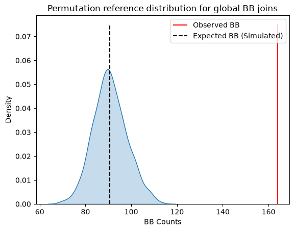
p-value (sim): 0.0010
jc.mean_bb, jc.bb
(np.float64(90.70170170170171), np.float64(164.0))
The simulations generate an average BB count of 90.7, while our observed BB join count was 164. Since the p-value from the simulation is below conventional significance levels, we would reject the null of complete spatial randomness in favor of spatial autocorrelation in market prices.
Takeaways
Join counts provide a global autocorrelation measure for binary variables. They are especially useful when the research question is about the clustering of categories rather than the similarity of continuous magnitudes. After establishing global clustering, the natural next step is to ask where those clusters occur, which is the focus of local spatial autocorrelation methods.