Global Spatial Autocorrelation Getis-Ord G¶

This notebook covers Getis-Ord statistics for identifying spatial concentrations of high or low values.

Learning goals¶

By the end of this notebook, you will be able to:

• compute the global \(G\) statistic and assess its significance

• explain how Getis-Ord \(G\) differs from Moran’s \(I\)

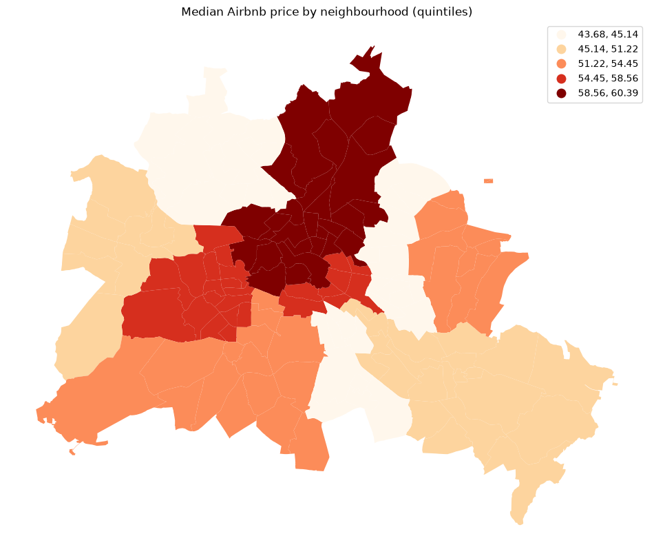
The substantive question is whether high Airbnb prices cluster spatially — and, if so, where those high-price hotspots are located.

import geopandas as gpd
import matplotlib.pyplot as plt
import numpy as np
import seaborn as sns
from libpysal import graph

import esda

Data preparation¶

We use the same Berlin neighborhood dataset as in the global Moran’s I and local Moran’s I notebooks so that results can be compared directly.

df = gpd.read_file("data/berlin-housing.gpkg")

fig, ax = plt.subplots(figsize=(12, 10))
df.plot(column="median_pri", scheme="Quantiles", k=5, cmap="OrRd", legend=True, ax=ax)
ax.set_axis_off()
ax.set_title("Median Airbnb price by neighbourhood (quintiles)")
plt.show()

Getis-Ord G¶

Moran’s I measures spatial autocorrelation by comparing each observation to its deviation from the global mean. A High-High cluster in Moran’s framework means both a neighborhood and its neighbors are above the mean.

Getis-Ord \(G\) takes a different approach: it measures spatial concentration of raw values. A high \(G\) means large values are co-located with other large values — a true hotspot. This can be better understood by examining the form of the statistic:

where \(x_i\) is the value for the variable \(x\) at location \(i\) of \(n\) locations, and \(w_{ij}\) is the spatial weight expressing the neighbor relationship between locations \(i\) and \(j\).

The expected value of \(G\) under the null hypothesis of no spatial association is:

Because \(G\) works with raw values rather than mean-centered deviations, it is particularly well-suited to detecting concentration of phenomena that are always non-negative (counts, prices, rates).

The global statistic \(G\) answers: is there a statistically significant overall concentration of high or low values?

# G requires binary (not row-standardised) weights
wq = graph.Graph.build_contiguity(df, rook=False)
y = df["median_pri"]

np.random.seed(12345)
g_global = esda.G(y, wq)
print(f"Observed G:   {g_global.G:.6f}")
print(f"Expected G:   {g_global.EG:.6f}")

Observed G:   0.040514
Expected G:   0.039671

The calculated value of the global statistic is above its expectation. Whether this difference is statistically significant, or larger than what could be due to a certain level of random chance, requires an inferential framework.

Inference¶

Inference about \(G\) uses the same general framework underlying Moran’s I, where the reference distribution can be based on analytical reasoning or permutation based.

To derive the analytical expected value and variance for statistical inference, we define the following structural constants based on the weights matrix \(W\):

• \(S_0 = \sum_{i=1}^n \sum_{j=1}^n w_{ij}\) (The sum of all spatial weights)

• \(S_1 = \frac{1}{2} \sum_{i=1}^n \sum_{j=1}^n (w_{ij} + w_{ji})^2\)

• \(S_2 = \sum_{i=1}^n \left( \sum_{j=1}^n w_{ij} + \sum_{j=1}^n w_{ji} \right)^2\)

We also define global moments of the attribute vector \(x\):

• \(W_0 = S_0\)

• The sample moments: \(D_1 = \sum_{i=1}^n x_i\), \(D_2 = \sum_{i=1}^n x_i^2\), \(D_3 = \sum_{i=1}^n x_i^3\), and \(D_4 = \sum_{i=1}^n x_i^4\).

Free Sampling (The Normality Assumption)¶

Expected Value¶

The expected value of \(G\) under free sampling depends entirely on the sample size \(n\) and the number of pairs, remaining independent of the empirical values of \(x\):

Variance¶

The mathematical variance under the normality assumption is structured as follows:

Non-Free Sampling (The Randomization Assumption)¶

Expected Value¶

Because the expectation across all permutations averages out the spatial structure, the expected value under randomization is identical to the free sampling expectation:

Variance¶

The variance under randomization must account for the exact empirical distribution of the data (incorporating higher-order sample moments \(D_3\) and \(D_4\)). The formula is conventionally expressed using a series of compounded variables:

Where \(E_R(G^2)\) is calculated as:

The structural data coefficients (\(A_1, A_2, A_3\)) isolate the interactions of the empirical array data:

And the denominator’s data product adjusts for the omission of the diagonal (\(i=j\)):

Asymptotic Inference (Z-score)¶

For practical execution, these analytical moments are translated into an asymptotic standard normal \(Z\)-score:

• Positive \(Z(G)\): Indicates a spatial cluster of high values (hot spots).

• Negative \(Z(G)\): Indicates a spatial cluster of low values (cold spots).

Because the randomization variance (\(Var_R(G)\)) natively accounts for extreme skewness and kurtosis common in positive non-negative values (like real estate prices or population counts), it is the default analytical configuration deployed for spatial boundary validation.

While computationally fast, the analytical approach relies on the assumption of normality which may not hold for small sample sizes or highly skewed data.

print(f"z-score:      {g_global.z_norm:.4f}")

z-score:      3.2702

print(f"p-value (norm): {g_global.p_norm:.4f}")

p-value (norm): 0.0005

Permutation-based inference¶

As with Moran’s \(I\), we can also assess the observed \(G\) against a reference distribution generated by randomly permuting attribute values while holding the spatial structure fixed.

sns.kdeplot(g_global.sim, fill=True)
plt.vlines(g_global.G, 0, plt.gca().get_ylim()[1] * 0.9, color="r", label="Observed G")
plt.vlines(
    g_global.EG,
    0,
    plt.gca().get_ylim()[1] * 0.9,
    color="k",
    linestyle="--",
    label="Expected G",
)
plt.xlabel("G statistic")
plt.legend()
plt.title("Permutation reference distribution for global G")
plt.show()

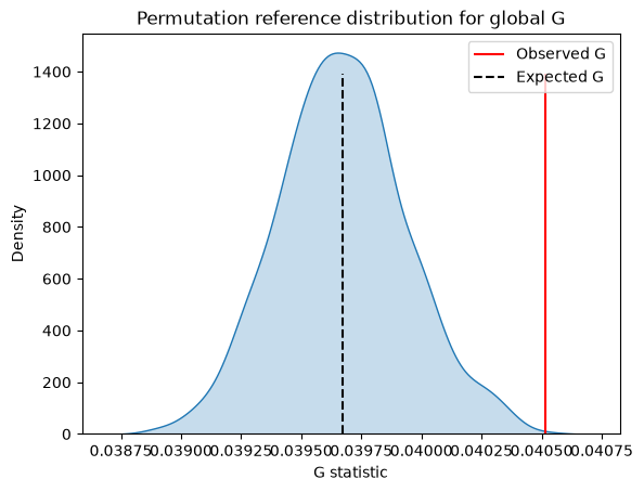
print(f"p-value (sim):  {g_global.p_sim:.4f}")

p-value (sim):  0.0020

Comparing Getis-Ord and Moran’s I results¶

The global \(G\) statistic captures concentrations of High-High values, as well as concentrations of Low-Low values, similar to the global Moran’s \(I\). The two methods can diverge when local variance is high — a neighborhood with very high prices surrounded by moderate prices may register as a spatial outlier in Moran but not a hotspot for \(G\).

Considerations¶

Two final points should be kept in mind when applying the global \(G\):

• Positivity Requirement: The values of \(x\) must be positive (\(x > 0\))

• The Zero Problem: The statistic is designed for ratio-scale data with a natural zero. If the data contains zeros or negative alues, the denominator (the sum of cross-products) can behave erratically, and the interpretation of “high” or “low” value clusters becomes mathematically unstable.

Takeaways¶

• Global G tests whether the entire study area has more concentration of high (or low) values than expected under spatial randomness.

• \(G\) does not capture negative spatial autocorrelation, in contrast to Moran’s I.