Using custom graphs
gwlearn’s geographically weighted modelling framework is built on top of libpysal.graph.Graph objects, which are typically generated on-the-fly based on the bandwidth and kernel specification. However, you can easily derive the graph in other way and use it wihtin the model, instead of relying on its limited distance and KNN builders.
Below is a basic example using linear regression and a graph redived from travel cost.
import geodatasets
import geopandas as gpd
import pandarm
from libpysal.graph import Graph

from gwlearn.linear_model import GWLinearRegression
Get some data you want to model. This dataset is assumed to contain both dependent and independent variables.
df = gpd.read_file(geodatasets.get_path("geoda Cincinnati"))
Downloading file 'walnuthills_updated.zip' from 'https://geodacenter.github.io/data-and-lab//data/walnuthills_updated.zip' to '/home/runner/.cache/geodatasets'.
Extracting 'walnuthills_updated' from '/home/runner/.cache/geodatasets/walnuthills_updated.zip' to '/home/runner/.cache/geodatasets/walnuthills_updated.zip.unzip'
Generate a pandarm.Network based on the extent of the dataset. This will automatically pull the data for street network from OpenStretMap and prepare a network that can be later queried. All points will be linked to this network and accessibility will be measured alongside its edges.
network = pandarm.Network.from_gdf(df)
Generating contraction hierarchies with 4 threads.
Setting CH node vector of size 8737
Setting CH edge vector of size 25826
Range graph removed 26324 edges of 51652
. 10% . 20% . 30% . 40% . 50% . 60% . 70% . 80% . 90% . 100%
/home/runner/micromamba/envs/py314-latest/lib/python3.14/site-packages/pandarm/loaders/osm.py:68: UserWarning: GeoDataFrame is stored in coordinate system PROJCS["Lambert_Conformal_Conic",GEOGCS["GCS_GRS 1980(IUGG, 1980)",DATUM["unknown",SPHEROID["GRS80",6378137,298.257222101]],PRIMEM["Greenwich",0],UNIT["Degree",0.0174532925199433]],PROJECTION["Lambert_Conformal_Conic_2SP"],PARAMETER["latitude_of_origin",38],PARAMETER["central_meridian",-82.5],PARAMETER["standard_parallel_1",40.0333333333333],PARAMETER["standard_parallel_2",38.7333333333333],PARAMETER["false_easting",1968500],PARAMETER["false_northing",0],UNIT["US survey foot",0.304800609601219,AUTHORITY["EPSG","9003"]],AXIS["Easting",EAST],AXIS["Northing",NORTH]] so the pandarm.Network will also be stored in this system
  warn(
Use the network to build a graph with a set distance threshold and a kernel transforming the actual distance to a distance decay weight.
G = Graph.build_travel_cost(
    df.set_geometry(df.representative_point()),
    network,
    threshold=1500,
    kernel="bisquare",
)
Check the properties of the resulting graph. You can see that on average, you have approximately 130 neighbors.
G.summary()
| Number of nodes: | 457 |
| Number of edges: | 60031 |
| Number of connected components: | 1 |
| Number of isolates: | 0 |
| Number of non-zero edges: | 60029 |
| Percentage of non-zero edges: | 28.74% |
| Number of asymmetries: | NA |
| Mean: | 131 | 25%: | 80 | |
| Standard deviation: | 60 | 50% | 137 | |
| Min: | 5 | 75%: | 181 | |
| Max: | 239 |
| Mean: | 0 | 25%: | 0 |
| Standard deviation: | 0 | 50% | 0 |
| Min: | 0 | 75%: | 1 |
| Max: | 1 |
| S0: | 20222 | GG: | 11840 |
| S1: | 23680 | G'G: | 11840 |
| S3: | 4548658 | G'G + GG: | 23680 |
[0, 1, 2, 3, 4, ...]
Fit the regression.
gwlr = GWLinearRegression(graph=G)
gwlr.fit(
    X=df[
        [
            "AGE_0_5",
            "AGE_5_9",
            "AGE_10_14",
            "AGE_15_19",
            "AGE_20_24",
            "AGE_25_34",
            "AGE_35_44",
            "AGE_45_54",
            "AGE_55_59",
            "AGE_60_64",
            "AGE_65_74",
            "AGE_75_84",
            "AGE_85",
        ]
    ],
    y=df["WHITE"],
)
GWLinearRegression(graph=<Graph of 457 nodes and 60029 nonzero edges (1 component, 0 isolates) indexed by
 [0, 1, 2, 3, 4, ...]>)
In a Jupyter environment, please rerun this cell to show the HTML representation or trust the notebook.
On GitHub, the HTML representation is unable to render, please try loading this page with nbviewer.org.
Parameters
| bandwidth | None | |
| fixed | False | |
| kernel | 'bisquare' | |
| include_focal | True | |
| graph | <Graph of 457...2, 3, 4, ...]> | |
| n_jobs | -1 | |
| fit_global_model | True | |
| strict | False | |
| keep_models | False | |
| temp_folder | None | |
| batch_size | None | |
| coplanar | 'raise' | |
| verbose | False |
Done. Now you can extract whatever the object contain. Like prediction.
gwlr.pred_
0      384.274447
1       11.771021
2       16.941807
3       17.726431
4       46.407925
          ...
452      5.427409
453      0.657813
454      0.260536
455      1.279797
456      2.558343
Length: 457, dtype: float64
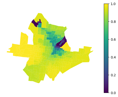
Or local R2.
gwlr.local_r2_
0      0.953835
1      0.974026
2      0.987761
3      0.974411
4      0.983311
         ...
452    0.790494
453    0.666854
454    0.709859
455    0.870750
456    0.855403
Length: 457, dtype: float64
That can be plotted.
df.plot(gwlr.local_r2_, legend=True, vmin=0, vmax=1).set_axis_off()