Bandwidth search
To find out the optimal bandwidth, gwlearn provides a BandwidthSearch class, which trains models on a range of bandwidths and selects the most optimal one.
import geopandas as gpd
from geodatasets import get_path

from gwlearn.linear_model import GWLinearRegression, GWLogisticRegression
from gwlearn.search import BandwidthSearch
Get sample data
gdf = gpd.read_file(get_path("geoda.south")).to_crs(5070)

gdf["point"] = gdf.representative_point()
gdf = gdf.set_geometry("point")

y = gdf["FH90"]
X = gdf.iloc[:, 9:15]
Downloading file 'south.zip' from 'https://geodacenter.github.io/data-and-lab//data/south.zip' to '/home/runner/.cache/geodatasets'.
Extracting 'south/south.gpkg' from '/home/runner/.cache/geodatasets/south.zip' to '/home/runner/.cache/geodatasets/south.zip.unzip'
Interval search
Interval search tests the model at a set interval. The default and recommended criterion for linear models is corrected Akaike’s information criterion (AICc).
search = BandwidthSearch(
    GWLinearRegression,
    fixed=False,
    n_jobs=-1,
    search_method="interval",
    min_bandwidth=50,
    max_bandwidth=1000,
    interval=100,
    criterion="aicc",
    verbose=True,
)
search.fit(
    X,
    y,
    geometry=gdf.geometry,
)
Bandwidth: 50.00, aicc: 7687.620
Bandwidth: 150.00, aicc: 7598.565
Bandwidth: 250.00, aicc: 7672.857
Bandwidth: 350.00, aicc: 7723.089
Bandwidth: 450.00, aicc: 7764.724
Bandwidth: 550.00, aicc: 7811.336
Bandwidth: 650.00, aicc: 7862.825
Bandwidth: 750.00, aicc: 7904.418
Bandwidth: 850.00, aicc: 7941.883
Bandwidth: 950.00, aicc: 7981.397
<gwlearn.search.BandwidthSearch at 0x7faebde2be00>
The scores_ series then contains the AICc, selected as the criterion, which can be plotted to see the change of the model performance as the bandwidth grows.
search.scores_.plot()
<Axes: >
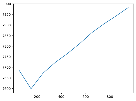
The optimal bandwidth is then the lowest one.
search.optimal_bandwidth_
150
Golden section
Alternatively, you can try to use the golden section algorithm that attempts to find the optimal bandwidth iteratively. However, note that there’s no guaratnee that it will find the globally optimal bandwidth as it may stick to the local minimum.
search = BandwidthSearch(
    GWLinearRegression,
    fixed=True,
    n_jobs=-1,
    search_method="golden_section",
    criterion="aicc",
    min_bandwidth=10_000,
    max_bandwidth=1_000_000,
    verbose=True,
)
search.fit(
    X,
    y,
    geometry=gdf.geometry,
)
Bandwidth: 388150.3, score: 7670.159
Bandwidth: 621849.7, score: 7770.628
Bandwidth: 243708.23, score: 7596.823
Bandwidth: 154442.07, score: 7912.455
Bandwidth: 298880.77, score: 7626.218
Bandwidth: 209613.32, score: 7617.231
Bandwidth: 264783.28, score: 7604.824
Bandwidth: 230686.59, score: 7597.453
Bandwidth: 251759.37, score: 7599.373
Bandwidth: 238735.76, score: 7596.182
Bandwidth: 235660.47, score: 7596.368
Bandwidth: 240634.23, score: 7596.262
Bandwidth: 237560.29, score: 7596.229
Bandwidth: 239460.08, score: 7596.185
<gwlearn.search.BandwidthSearch at 0x7faebdb02e90>
You can see how the agorithm searches and iteratively gets closer to the optimum.
search.optimal_bandwidth_
np.float64(238735.7582789531)
Other metrics
By default, BandwidthSearch computes AICc, AIC and BIC for linear models, available through metrics_.
search.metrics_
| aicc | aic | bic | |
|---|---|---|---|
| 388150.300000 | 7670.159314 | 7650.730706 | 8238.208833 |
| 621849.700000 | 7770.627977 | 7766.321405 | 8047.693794 |
| 243708.229909 | 7596.823008 | 7497.313206 | 8762.156146 |
| 154442.070091 | 7912.454856 | 7355.237895 | 9995.188728 |
| 298880.767422 | 7626.217681 | 7578.766844 | 8477.096909 |
| 209613.319310 | 7617.230987 | 7443.545102 | 9065.985674 |
| 264783.280267 | 7604.823570 | 7531.986411 | 8628.488146 |
| 230686.589297 | 7597.453089 | 7475.433826 | 8862.323769 |
| 251759.367217 | 7599.373132 | 7511.192286 | 8708.266105 |
| 238735.758279 | 7596.181669 | 7488.668425 | 8798.649792 |
| 235660.465361 | 7596.367751 | 7483.564238 | 8822.281852 |
| 240634.225285 | 7596.262234 | 7491.905192 | 8784.335011 |
| 237560.292439 | 7596.229247 | 7486.713835 | 8807.668987 |
| 239460.075156 | 7596.184987 | 7489.889063 | 8793.138119 |
You can also ask for a log loss and even use it as a criterion for the selection. This is useful when comparing classification models with varying prediction rate (you can also retrieve that for each bandwidth) or when using non-linear models, where MAE or RMSE should be used instead of AICc.
search = BandwidthSearch(
    GWLogisticRegression,
    fixed=False,
    n_jobs=-1,
    search_method="interval",
    min_bandwidth=50,
    max_bandwidth=1000,
    interval=200,
    metrics=["log_loss", "prediction_rate"],
    criterion="log_loss",
    verbose=True,
)
search.fit(
    X,
    y > y.median(),  # simulate binary categorical variable
    geometry=gdf.geometry,
)
Bandwidth: 50.00, log_loss: 0.276
Bandwidth: 250.00, log_loss: 0.376
Bandwidth: 450.00, log_loss: 0.413
Bandwidth: 650.00, log_loss: 0.437
Bandwidth: 850.00, log_loss: 0.454
<gwlearn.search.BandwidthSearch at 0x7faebdda3610>
Log loss is then part of the metrics.
search.metrics_
| aicc | aic | bic | log_loss | prediction_rate | |
|---|---|---|---|---|---|
| 50 | 1378.952921 | 1119.216533 | 2551.160956 | 0.275782 | 0.682011 |
| 250 | 1263.263762 | 1249.800971 | 1741.819969 | 0.376227 | 1.000000 |
| 450 | 1275.477037 | 1271.315792 | 1547.948404 | 0.412885 | 1.000000 |
| 650 | 1308.279791 | 1306.304157 | 1497.258268 | 0.436826 | 1.000000 |
| 850 | 1337.858308 | 1336.720382 | 1481.487638 | 0.453824 | 1.000000 |
And is reported directly as score as it is set as the criterion.
search.scores_.plot()
<Axes: >
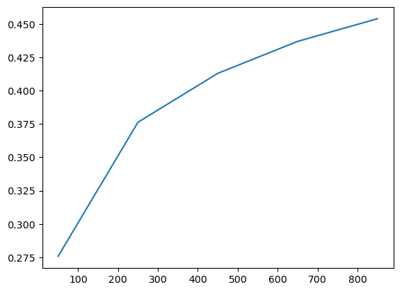
As a result, the optimal bandwidth is derived directly from it.
search.optimal_bandwidth_
50