Simulating Population Groups Distributed Randomly in Space

For conducting single-value inference, the segregation package offers several techniques for generating random population distributions that respect the characteristics of an input dataset. This notebook walks through the assumptions and outputs of each approach using the Sacramento demonstration dataset bundled with libpysal.

TL;DR

• evenness includes group-level variation

• systematic includes unit-level variation

• individual permutation includes neither

%load_ext watermark
%watermark -a 'eli knaap' -v -d -u -p segregation,geopandas,libpysal

Author: eli knaap

Last updated: 2026-09-04

Python implementation: CPython
Python version       : 3.14.7
IPython version      : 9.17.1

segregation: 2.5.6.dev83+g2e095ced1
geopandas  : 1.1.4
libpysal   : 4.15.0

import numpy as np
import geopandas as gpd
import matplotlib.pyplot as plt

from libpysal.examples import load_example
from segregation.singlegroup import Gini
from segregation.multigroup import MultiInfoTheory
from segregation.inference import (
    SingleValueTest,
    simulate_evenness,
    simulate_person_permutation,
    simulate_systematic_randomization,
    simulate_null,
)

sacramento = gpd.read_file(load_example("Sacramento1").get_path("sacramentot2.shp"))
sacramento = sacramento.to_crs(sacramento.estimate_utm_crs())

We focus on the Black population (BLACK) relative to the total population (TOT_POP) of each tract.

sacramento["BLACK"].sum()

np.int64(122022)

sacramento["TOT_POP"].sum()

np.int64(1796857)

sacramento["BLACK"].sum() / sacramento["TOT_POP"].sum()

np.float64(0.06790857591895182)

gini = Gini(sacramento, group_pop_var="BLACK", total_pop_var="TOT_POP")

Evenness

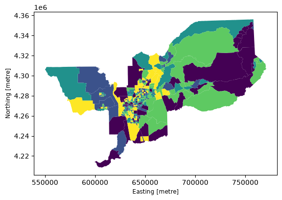
Evenness takes draws from the population of each unit, with the probability of choosing the focal group equal to its regional share (locations drawing from distributions of population groups).

# the region-wide share of the Black population
sacramento["BLACK"].sum() / sacramento["TOT_POP"].sum()

np.float64(0.06790857591895182)

sacramento[["TOT_POP"]].reset_index(drop=True).head()

	TOT_POP
0	5501
1	2072
2	3633
3	1683
4	5794

For the first tract, one draw is taken per resident; on each draw the probability that the resident belongs to the focal group equals the region-wide share computed above.

evenness = simulate_evenness(sacramento, group="BLACK", total="TOT_POP")

evenness

	BLACK	TOT_POP	geometry
0	391	5501	POLYGON ((740409.853 4338451.728, 740199.864 4...
1	140	2072	POLYGON ((753400.378 4347151.08, 753395.816 43...
2	212	3633	POLYGON ((758318.262 4352123.456, 758319.774 4...
3	99	1683	POLYGON ((750839.595 4342678.807, 750805.84 43...
4	370	5794	POLYGON ((670062.02 4311030.409, 670133.819 43...
...	...	...	...
398	492	7381	POLYGON ((653551.937 4240067.267, 653554.274 4...
399	224	3123	POLYGON ((649291.986 4235408.766, 649242.118 4...
400	472	6843	POLYGON ((647004.438 4239439.343, 647018.86 42...
401	124	1859	POLYGON ((649798.098 4234453.137, 649774.513 4...
402	110	1934	POLYGON ((599784.769 4213752.016, 599769.473 4...

403 rows × 3 columns

evenness.plot("BLACK", scheme="quantiles")

<Axes: >

evenness["BLACK"].sum()

np.int64(122007)

evenness["BLACK"].sum() == sacramento["BLACK"].sum()

np.False_

evenness["BLACK"].sum() / evenness["TOT_POP"].sum()

np.float64(0.06790022800924057)

sacramento["BLACK"].sum() / sacramento["TOT_POP"].sum()

np.float64(0.06790857591895182)

evenness["BLACK"].sum() / evenness["TOT_POP"].sum() == sacramento["BLACK"].sum() / sacramento["TOT_POP"].sum()

np.False_

evenness["TOT_POP"].sum() == sacramento["TOT_POP"].sum()

np.True_

np.array_equal(evenness["TOT_POP"].values, sacramento["TOT_POP"].values)

True

We haven’t changed the total population in each unit or in the region, but we have changed the number of people in the focal group marginally.

Systematic Randomization

The systematic approach takes draws from the regional population of each group, with the probability of choosing a geographic unit equal to the share of the region’s population that currently lives there (people drawing from a distribution of locations).

sacramento["BLACK"].sum()

np.int64(122022)

(sacramento["TOT_POP"] / sacramento["TOT_POP"].sum()).reset_index(drop=True).head()

0    0.003061
1    0.001153
2    0.002022
3    0.000937
4    0.003225
Name: TOT_POP, dtype: float64

For each member of the focal group, the probability of being placed in a given tract equals that tract’s share of the total population (shown above for the first few tracts).

systematic = simulate_systematic_randomization(
    sacramento, group="BLACK", total="TOT_POP"
)

systematic

	index	geometry	BLACK	other_group_pop	TOT_POP
0	0	POLYGON ((740409.853 4338451.728, 740199.864 4...	377	5171	5548
1	1	POLYGON ((753400.378 4347151.08, 753395.816 43...	126	1863	1989
2	2	POLYGON ((758318.262 4352123.456, 758319.774 4...	244	3347	3591
3	3	POLYGON ((750839.595 4342678.807, 750805.84 43...	128	1614	1742
4	4	POLYGON ((670062.02 4311030.409, 670133.819 43...	383	5332	5715
...	...	...	...	...	...
398	398	POLYGON ((653551.937 4240067.267, 653554.274 4...	472	6920	7392
399	399	POLYGON ((649291.986 4235408.766, 649242.118 4...	205	2901	3106
400	400	POLYGON ((647004.438 4239439.343, 647018.86 42...	466	6333	6799
401	401	POLYGON ((649798.098 4234453.137, 649774.513 4...	142	1729	1871
402	402	POLYGON ((599784.769 4213752.016, 599769.473 4...	126	1858	1984

403 rows × 5 columns

systematic["BLACK"].sum()

np.int64(122022)

systematic["BLACK"].sum() == sacramento["BLACK"].sum()

np.True_

systematic["BLACK"].sum() / systematic["TOT_POP"].sum() == sacramento["BLACK"].sum() / sacramento["TOT_POP"].sum()

np.True_

np.array_equal(systematic["TOT_POP"].values, sacramento["TOT_POP"].values)

False

We haven’t changed the total number of people in each group, but we have changed the total number of people in each unit.

Individual-level Permutation

Individual-level permutation doesn’t take draws from a probability distribution, but instead randomizes which unit each person lives in.

permutation = simulate_person_permutation(
    sacramento, group="BLACK", total="TOT_POP"
)

permutation["BLACK"].sum()

np.int64(122022)

permutation["BLACK"].sum() == sacramento["BLACK"].sum()

np.True_

permutation["BLACK"].sum() / permutation["TOT_POP"].sum() == sacramento["BLACK"].sum() / sacramento["TOT_POP"].sum()

np.True_

We haven’t changed the total number of people in any group, or the total population in any unit; we’ve only randomized which unit each person lives in.

Simulating Null Distributions

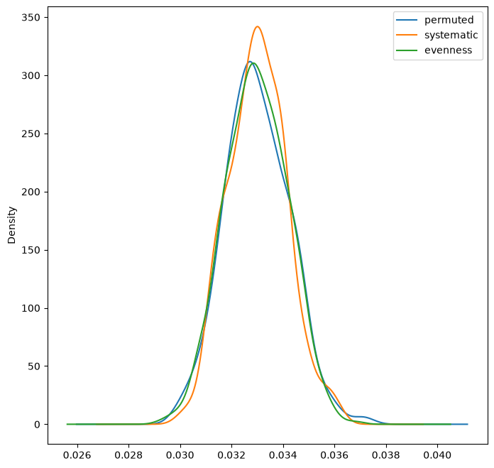
simulate_null generates a series of simulated segregation statistics (in parallel) using the randomization functions described above. Those simulated values can then serve as a reference distribution to test the hypothesis of “no segregation”.

groups = ["BLACK", "WHITE", "ASIAN", "HISP"]

G = Gini(sacramento, group_pop_var="BLACK", total_pop_var="TOT_POP")

H = MultiInfoTheory(sacramento, groups=groups)

G.statistic

0.6361755332635235

H.statistic

np.float64(0.17101602978588876)

Single Group

G_even = simulate_null(seg_class=G, sim_func=simulate_evenness)

G_systematic = simulate_null(seg_class=G, sim_func=simulate_systematic_randomization)

G_permuted = simulate_null(seg_class=G, sim_func=simulate_person_permutation)

fig, ax = plt.subplots(figsize=(8, 8))
for series, label in [
    (G_permuted, "permuted"),
    (G_systematic, "systematic"),
    (G_even, "evenness"),
]:
    series.name = label
    series.plot(kind="kde", ax=ax, legend=True)

Multi Group

H_even = simulate_null(seg_class=H, sim_func=simulate_evenness)

H_systematic = simulate_null(seg_class=H, sim_func=simulate_systematic_randomization)

H_permuted = simulate_null(seg_class=H, sim_func=simulate_person_permutation)

fig, ax = plt.subplots(figsize=(8, 8))
for series, label in [
    (H_permuted, "permuted"),
    (H_systematic, "systematic"),
    (H_even, "evenness"),
]:
    series.name = label
    series.plot(kind="kde", ax=ax, legend=True)

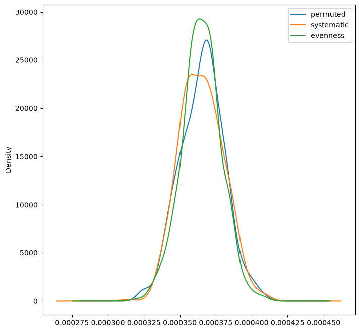
Despite their different methods, all three approaches simulate similar distributions, but they differ with respect to how and in which dimensions the randomization occurs. As with Boisso et al., the distribution is not centered on 0. In other cases, such as when minority populations are small or highly unbalanced among multiple groups, it is possible that the different randomization methods could diverge to simulate different distributions.