Single-group Segregation Indices¶

[1]:

%load_ext watermark
%watermark -a 'eli knaap' -v -d -u -p segregation,geopandas,libpysal,pandana

Author: eli knaap

Last updated: 2021-05-11

Python implementation: CPython
Python version       : 3.9.2
IPython version      : 7.23.1

segregation: 2.0.0
geopandas  : 0.9.0
libpysal   : 4.3.0
pandana    : 0.6.1

Single-group indices are calculated using the singlegroup module

Data Prep¶

[2]:

import geopandas as gpd
import matplotlib.pyplot as plt
from libpysal.examples import load_example

[3]:

# read in sacramento data from libpysal and reproject into an appropriate CRS
sacramento = gpd.read_file(load_example("Sacramento1").get_path("sacramentot2.shp"))
sacramento = sacramento.to_crs(sacramento.estimate_utm_crs())

[4]:

sacramento.head()

[4]:

	FIPS	MSA	TOT_POP	POP_16	POP_65	WHITE	BLACK	ASIAN	HISP	MULTI_RA	...	EMP_FEM	OCC_MAN	OCC_OFF1	OCC_INFO	HH_INC	POV_POP	POV_TOT	HSG_VAL	POLYID	geometry
0	06061022001	Sacramento	5501	1077	518	4961	29	82	336	31	...	1187	117	663.0	42	52941	5461	470	225900	1	POLYGON ((740409.853 4338451.728, 740199.864 4...
1	06061020106	Sacramento	2072	396	109	1603	0	28	391	41	...	522	38	229.0	19	51958	2052	160	249300	2	POLYGON ((753400.378 4347151.080, 753395.816 4...
2	06061020107	Sacramento	3633	911	126	1624	9	0	1918	41	...	698	86	197.0	0	32992	3604	668	175900	3	POLYGON ((758318.262 4352123.456, 758319.774 4...
3	06061020105	Sacramento	1683	281	154	1564	0	55	60	4	...	519	5	256.0	6	54556	1683	116	302300	4	POLYGON ((750839.595 4342678.807, 750805.840 4...
4	06061020200	Sacramento	5794	1278	830	5185	17	13	251	229	...	1260	155	506.0	59	50815	5771	342	167300	5	POLYGON ((670062.020 4311030.409, 670133.819 4...

5 rows × 31 columns

[5]:

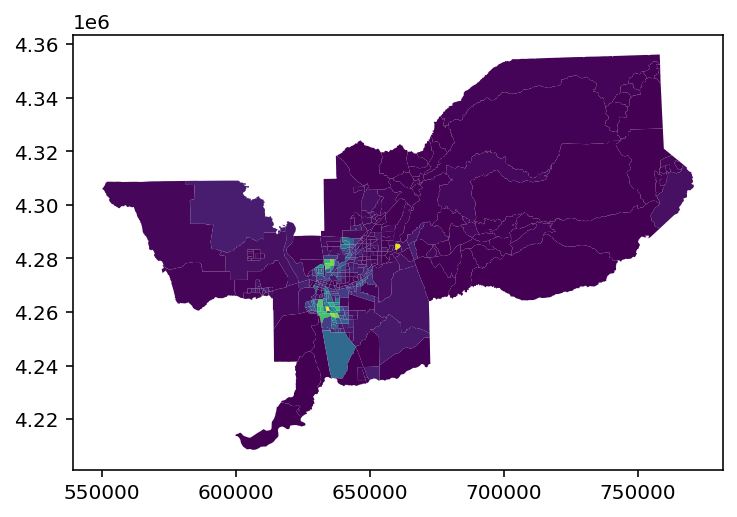
sacramento.plot('BLACK')

[5]:

<AxesSubplot:>

../_images/notebooks_01_singlegroup_indices_7_1.png

Aspatial Segregation Indices¶

To compute an aspatial segregation index, pass a dataframe, a group population variable, and total population variable to the index’s class

[6]:

from segregation.singlegroup import Dissim

[7]:

dissim = Dissim(sacramento, group_pop_var='BLACK',
                total_pop_var='TOT_POP')

The statistic attribute holds the value of the segregation index, and the data attribute holds the data used to calculate the index

[8]:

dissim.statistic

[8]:

0.4883394024705785

[9]:

dissim.data.head()

[9]:

	BLACK	TOT_POP	geometry
0	29	5501	POLYGON ((740409.853 4338451.728, 740199.864 4...
1	0	2072	POLYGON ((753400.378 4347151.080, 753395.816 4...
2	9	3633	POLYGON ((758318.262 4352123.456, 758319.774 4...
3	0	1683	POLYGON ((750839.595 4342678.807, 750805.840 4...
4	17	5794	POLYGON ((670062.020 4311030.409, 670133.819 4...

Spatial Segregation Indices¶

For calculating spatial segregation indices, the package implements two classes of indices: spatially-explicit and spatially-implicit.

Spatially-explicit indices are those for which space was a formal consideration in the index’s original formulation, whereas spatially-implicit indices are developed using the logic of Reardon and O’Sulivan.

For the latter,(otherwise called generalized spatial segregation indices) the package can incorporate spatial relationships represented by either a `libpysal.W <https://pysal.org/libpysal/api.html>`__ weights object or a `pandana.Network <http://udst.github.io/pandana/network.html>`__ network object, which means generalized spatial segregation indices can be computed according to many different spatial relationships which could include contiguity, distance, or network connectivity. This flexibility is particularly useful for specifying appropriate “neighborhood” definitions for different types of input data (which could be, e.g. housing units, census tracts, or counties)

For spatially-explicit indices, they can be called like any other, though some may have additional arguments:

[10]:

from segregation.singlegroup import AbsoluteCentralization, Gini

[11]:

cent = AbsoluteCentralization(sacramento, group_pop_var='BLACK',
                              total_pop_var='TOT_POP')

[12]:

cent.statistic

[12]:

0.8491771822066525

Euclidian distance based measures¶

For generalized spatial indices, a distance parameter can be passed to the index of choice. Under the hood, the input data will be passed through a kernel function with the distance parameter as the kernel bandwidth.

(note in this case because the CRS of the sacramento dataframe is UTM, the units are in meters)

[13]:

# aspatial gini index
aspatial_gini = Gini(sacramento, group_pop_var='BLACK',
                     total_pop_var='TOT_POP')

[14]:

# generalized spatial gini index
gen_spatialgini = Gini(sacramento, group_pop_var='BLACK',
                       total_pop_var='TOT_POP', distance=2000)

[15]:

gen_spatialgini.statistic

[15]:

0.5368102768280784

[16]:

aspatial_gini.statistic

[16]:

0.6361755332635235

Examining the data attribute of the fitted index shows how the input data are transformed

[17]:

# kernelized data
gen_spatialgini.data.plot('BLACK')

[17]:

<AxesSubplot:>

../_images/notebooks_01_singlegroup_indices_28_1.png

[18]:

# original data
sacramento.plot('BLACK')

[18]:

<AxesSubplot:>

../_images/notebooks_01_singlegroup_indices_29_1.png

Network distance based measures¶

Instead of a euclidian distance-based kernel, each generalized spatial segregation index can be calculated using accssibility analysis on a transportation network instead. Since people can’t fly, using a travel network to measure spatial distances is more conceptually pure to the spirit of segregation indices

[19]:

import pandana as pdna

A network can be created using the urbanaccess package, or the built-in get_osm_network function from the segregation.util module. Alternatively, metropolitan-scale networks from OpenStreetMap are also available in the CGS quilt bucket (named by CBSA FIPS code)

[ ]:

[20]:

net = pdna.Network.from_hdf5('../40900.h5')

[21]:

network_spatialgini = Gini(sacramento, group_pop_var='BLACK',
                           total_pop_var='TOT_POP', distance=2000,
                           network=net, decay='linear')

Comparing spatial gini indices based on straight-line distance versus network distance:

[22]:

network_spatialgini.statistic

[22]:

0.5848616778202473

[23]:

gen_spatialgini.statistic

[23]:

0.5368102768280784

The segregation statistic using network distance to construct neighborhoods is higher than using the one using unrestricted euclidian distance

Batch-Computing Single-Group Measures¶

To compute all single group indices in one go, the package provides a wrapper function in the batch module

[24]:

from segregation.batch import batch_compute_singlegroup

[25]:

all_singlegroup = batch_compute_singlegroup(sacramento, group_pop_var='BLACK', total_pop_var='TOT_POP')

[26]:

all_singlegroup

[26]:

	Statistic
Name
AbsoluteCentralization	0.849177
AbsoluteClustering	0.117545
AbsoluteConcentration	0.981443
Atkinson	0.365947
BiasCorrectedDissim	0.487694
BoundarySpatialDissim	0.450074
ConProf	0.112752
CorrelationR	0.101027
Delta	0.907277
DensityCorrectedDissim	0.335178
Dissim	0.488339
DistanceDecayInteraction	0.841137
DistanceDecayIsolation	0.160247
Entropy	0.112068
Gini	0.636176
Interaction	0.837925
Isolation	0.162075
MinMax	0.656220
ModifiedDissim	0.476238
ModifiedGini	0.623809
PARDissim	0.481833
RelativeCentralization	0.076906
RelativeClustering	1.626559
RelativeConcentration	0.778755
SpatialDissim	0.446272
SpatialProxProf	0.115984
SpatialProximity	1.106990

[ ]: