This page was generated from user-guide/weights/Raster_awareness_API.ipynb.
Interactive online version:
![]()
Raster awareness API
This notebook will give an overview of newly developed raster interface. We’ll cover basic usage of the functionality offered by the interface which mainly involves:
converting
xarray.DataArrayobject to the PySAL’s weights object (libpysal.weights.W/WSP).going back to the
xarray.DataArrayfrom weights object.
using different datasets:
with missing values.
with multiple layers.
with non conventional dimension names.
[1]:
%matplotlib inline

import matplotlib.pyplot as plt
import numpy as np
import xarray as xr
from esda import Moran_Local
from splot import libpysal as splot

from libpysal.weights import Queen, Rook, raster
Loading Data
The interface only accepts ``xarray.DataArray``, this can be easily obtained from raster data format using xarray’s I/O functionality which can read from a variety of data formats some of them are listed below:
GDAL Raster Formats via
open_rasteriomethod.NetCDF via
open_datasetmethod.
In this notebook we’ll work with NetCDF and GeoTIFF data.
Using xarray example dataset
First lets load up a netCDF dataset offered by xarray.
[2]:
# -> returns a xarray.Dataset object
ds = xr.tutorial.open_dataset("air_temperature.nc")
da = ds["air"]  # we'll use the "air" data variable for further analysis
print(da)
<xarray.DataArray 'air' (time: 2920, lat: 25, lon: 53)>
[3869000 values with dtype=float32]
Coordinates:
  * lat      (lat) float32 75.0 72.5 70.0 67.5 65.0 ... 25.0 22.5 20.0 17.5 15.0
  * lon      (lon) float32 200.0 202.5 205.0 207.5 ... 322.5 325.0 327.5 330.0
  * time     (time) datetime64[ns] 2013-01-01 ... 2014-12-31T18:00:00
Attributes:
    long_name:     4xDaily Air temperature at sigma level 995
    units:         degK
    precision:     2
    GRIB_id:       11
    GRIB_name:     TMP
    var_desc:      Air temperature
    dataset:       NMC Reanalysis
    level_desc:    Surface
    statistic:     Individual Obs
    parent_stat:   Other
    actual_range:  [185.16 322.1 ]
xarray’s data structures like Dataset and DataArray provides pandas like functionality for multidimensional-array or ndarray.
In our case we’ll mainly deal with DataArray, we can see above that the da holds the data for air temperature, it has 2 dims coordinate dimensions x and y, and it’s layered on time dimension so in total 3 dims (time, lat, lon).
We’ll now group da by month and take average over the time dimension
[3]:
da = da.groupby("time.month").mean()
print(da.coords)  # as a result time dim is replaced by month
Coordinates:
  * lat      (lat) float32 75.0 72.5 70.0 67.5 65.0 ... 25.0 22.5 20.0 17.5 15.0
  * lon      (lon) float32 200.0 202.5 205.0 207.5 ... 322.5 325.0 327.5 330.0
  * month    (month) int64 1 2 3 4 5 6 7 8 9 10 11 12
[4]:
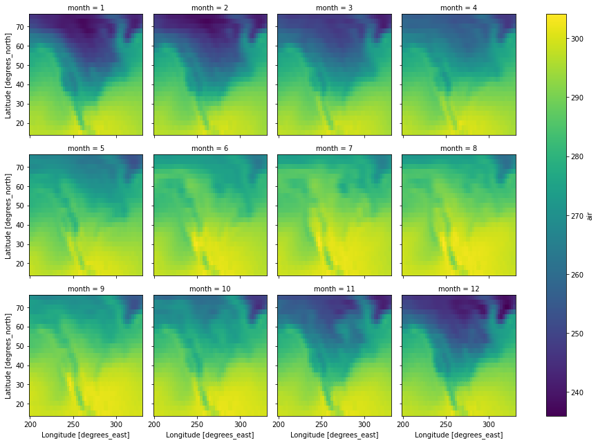
# let's plot over month, each facet will represent
# the mean air temperature in a given month.
da.plot(
    col="month",
    col_wrap=4,
)
[4]:
<xarray.plot.facetgrid.FacetGrid at 0x7f68f71b8100>
We can use from_xarray method from the contiguity classes like Rook and Queen, and also from KNN.
This uses a util function in raster.py file called da2W, which can also be called directly to build W object, similarly da2WSP for building WSP object.
Weight builders (``from_xarray``, ``da2W``, ``da2WSP``) can recognise dimensions belonging to this list ``[band, time, lat, y, lon, x]``, if any of the dimension in the ``DataArray`` does not belong to the mentioned list then we need to pass a dictionary (specifying that dimension’s name) to the weight builder.
e.g. dims dictionary:
>>> da.dims                  # none of the dimension belong to the default dimension list
('year', 'height', 'width')
>>> coords_labels = {                 # dimension values should be properly aligned with the following keys
        "z_label": "year",
        "y_label": "height",
        "x_label": "width"
    }
[5]:
coords_labels = {}
# since month does not belong to the default list we
# need to pass it using a dictionary
coords_labels["z_label"] = "month"
w_queen = Queen.from_xarray(
    da, z_value=12, coords_labels=coords_labels, sparse=False
)  # We'll use data from 12th layer (in our case layer=month)
/data/GSoC/libpysal/libpysal/weights/raster.py:119: UserWarning: You are trying to build a full W object from xarray.DataArray (raster) object. This computation can be very slow and not scale well. It is recommended, if possible, to instead build WSP object, which is more efficient and faster. You can do this by using da2WSP method.
  warn(
index is a newly added attribute to the weights object, this holds the multi-indices of the non-missing values belonging to pandas.Series created from the passed DataArray, this series can be easily obtained using DataArray.to_series() method.
[6]:
w_queen.index[:5] # indices are aligned to the ids of the weight object
[6]:
MultiIndex([(12, 75.0, 200.0),
            (12, 75.0, 202.5),
            (12, 75.0, 205.0),
            (12, 75.0, 207.5),
            (12, 75.0, 210.0)],
           names=['month', 'lat', 'lon'])
We can then obtain raster data by converting the DataArray to Series and then using indices from index attribute to get non-missing values by subsetting the Series.
[7]:
data = da.to_series()[w_queen.index]
We now have the required data for further analysis (we can now use methods such as ESDA/spatial regression), for this example let’s compute a local Moran statistic for the extracted data.
[8]:
# Quickly computing and loading a LISA
np.random.seed(12345)
lisa = Moran_Local(np.array(data, dtype=np.float64), w_queen)
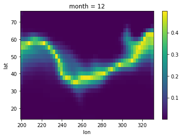
After getting our calculated results it’s time to store them back to the DataArray, we can use w2da function directly to convert the W object back to DataArray.
Your use case might differ but the steps for using the interface will be similar to this example.
[9]:
# Converting obtained data back to DataArray
moran_da = raster.w2da(
    lisa.p_sim, w_queen
)  # w2da accepts list/1d array/pd.Series and a weight object aligned to passed data
print(moran_da)
<xarray.DataArray (month: 1, lat: 25, lon: 53)>
array([[[0.018, 0.001, 0.001, ..., 0.001, 0.001, 0.001],
        [0.001, 0.001, 0.001, ..., 0.001, 0.001, 0.001],
        [0.003, 0.001, 0.001, ..., 0.001, 0.001, 0.001],
        ...,
        [0.002, 0.001, 0.001, ..., 0.001, 0.001, 0.003],
        [0.001, 0.001, 0.001, ..., 0.001, 0.001, 0.003],
        [0.002, 0.001, 0.001, ..., 0.001, 0.002, 0.006]]])
Coordinates:
  * month    (month) int64 12
  * lat      (lat) float64 75.0 72.5 70.0 67.5 65.0 ... 25.0 22.5 20.0 17.5 15.0
  * lon      (lon) float64 200.0 202.5 205.0 207.5 ... 322.5 325.0 327.5 330.0
[10]:
moran_da.plot()
[10]:
<matplotlib.collections.QuadMesh at 0x7f68f4044940>
Using local NetCDF dataset
In the earlier example we used an example dataset from xarray for building weights object. Additonally, we had to pass the custom layer name to the builder.
In this small example we’ll build KNN distance weight object using a local NetCDF dataset with different dimensions names which doesn’t belong to the default list of dimensions.
We’ll also see how to speed up the reverse journey (from weights object to DataArray) by passing prebuilt coords and attrs to w2da method.
[11]:
# Lets load a netCDF Surface dataset
ds = xr.open_dataset(
    "ECMWF_ERA-40_subset.nc"
)  # After loading netCDF dataset we obtained a xarray.Dataset object
print(ds)  # This Dataset object containes several data variables
<xarray.Dataset>
Dimensions:    (latitude: 73, longitude: 144, time: 62)
Coordinates:
  * longitude  (longitude) float32 0.0 2.5 5.0 7.5 ... 350.0 352.5 355.0 357.5
  * latitude   (latitude) float32 90.0 87.5 85.0 82.5 ... -85.0 -87.5 -90.0
  * time       (time) datetime64[ns] 2002-07-01T12:00:00 ... 2002-07-31T18:00:00
Data variables:
    tcw        (time, latitude, longitude) float32 ...
    tcwv       (time, latitude, longitude) float32 ...
    lsp        (time, latitude, longitude) float32 ...
    cp         (time, latitude, longitude) float32 ...
    msl        (time, latitude, longitude) float32 ...
    blh        (time, latitude, longitude) float32 ...
    tcc        (time, latitude, longitude) float32 ...
    p10u       (time, latitude, longitude) float32 ...
    p10v       (time, latitude, longitude) float32 ...
    p2t        (time, latitude, longitude) float32 ...
    p2d        (time, latitude, longitude) float32 ...
    e          (time, latitude, longitude) float32 ...
    lcc        (time, latitude, longitude) float32 ...
    mcc        (time, latitude, longitude) float32 ...
    hcc        (time, latitude, longitude) float32 ...
    tco3       (time, latitude, longitude) float32 ...
    tp         (time, latitude, longitude) float32 ...
Attributes:
    Conventions:  CF-1.0
    history:      2004-09-15 17:04:29 GMT by mars2netcdf-0.92
Out of 17 data variables we’ll use p2t for our analysis. This will give us our desired DataArray object da, we will further group da by day, taking average over the time dimension.
[12]:
# this will give us the required DataArray with p2t
# (2 metre temperature) data variable
da = ds["p2t"]
da = da.groupby("time.day").mean()
print(da.dims)
('day', 'latitude', 'longitude')
We can see that the none of dimensions of ``da`` matches with the default dimensions (``[band, time, lat, y, lon, x]``)
This means we have to create a dictionary mentioning the dimensions and ship it to weight builder, similar to our last example.
[13]:
coords_labels = {}
coords_labels["y_label"] = "latitude"
coords_labels["x_label"] = "longitude"
coords_labels["z_label"] = "day"
w_rook = Rook.from_xarray(da, z_value=13, coords_labels=coords_labels, sparse=True)
[14]:
data = da.to_series()[
    w_rook.index
]  # we derived the data from DataArray similar to our last example
In the last example we only passed the data values and weight object to w2da method, which then created the necessary coords to build our required DataArray. This process can be speed up by passing coords from the existing DataArray da which we used earlier.
Along with coords we can also pass attrs of the same DataArray this will help w2da to retain all the properties of original DataArray.
Let’s compare the DataArray returned by w2da and original DataArray. For this we’ll ship the derived data straight to w2da without any statistical analysis.
[15]:
da1 = raster.wsp2da(data, w_rook, attrs=da.attrs, coords=da[12:13].coords)
xr.DataArray.equals(
    da[12:13], da1
)  # method to compare 2 DataArray, if true then w2da was successfull
[15]:
True
Using local GeoTIFF dataset
Up until now we’ve only played with netCDF datasets but in this example we’ll use a raster.tif file to see how interface interacts with it. We’ll also see how these methods handle missing data.
Unlike earlier we’ll use weight builder methods from raster.py, which we can call directly. Just a reminder that from_xarray uses methods from raster.py and therefore only difference exists in the API.
To access GDAL Raster Formats xarray offers open_rasterio method which uses rasterio as backend. It loads metadata, coordinate values from the raster file and assign them to the DataArray.
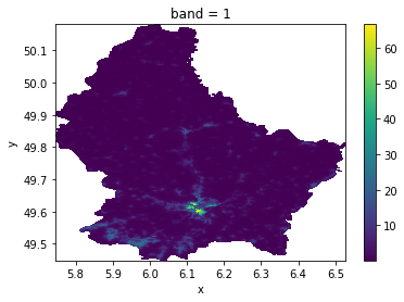
[16]:
# Loading raster data with missing values
da = xr.open_rasterio("/data/Downloads/lux_ppp_2019.tif")
print(da)
<xarray.DataArray (band: 1, y: 880, x: 940)>
[827200 values with dtype=float32]
Coordinates:
  * band     (band) int64 1
  * y        (y) float64 50.18 50.18 50.18 50.18 ... 49.45 49.45 49.45 49.45
  * x        (x) float64 5.745 5.746 5.747 5.747 ... 6.525 6.526 6.527 6.527
Attributes:
    transform:      (0.0008333333297872345, 0.0, 5.744583325, 0.0, -0.0008333...
    crs:            +init=epsg:4326
    res:            (0.0008333333297872345, 0.0008333333295454553)
    is_tiled:       0
    nodatavals:     (-99999.0,)
    scales:         (1.0,)
    offsets:        (0.0,)
    AREA_OR_POINT:  Area
[17]:
da.where(
    da.values > da.attrs["nodatavals"][0]
).plot()  # we can see that the DataArray contains missing values.
[17]:
<matplotlib.collections.QuadMesh at 0x7f68ef4c5ca0>
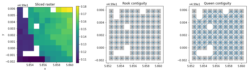
We’ll look at how weight builders handle missing values. Firstly we’ll slice the DataArray to reduce overall size for easier visualization.
This time we’ll create WSP object using da2WSP method inside raster.py. Since our DataArray is single banded and all of its dimensions belong to the default list, we only have to ship the DataArray and the type of contiguity we need.
[18]:
# Slicing the dataarray
da_s = da[:, 330:340, 129:139]
w_queen = raster.da2WSP(da_s)  # default contiguity is queen
w_rook = raster.da2WSP(da_s, "rook")
After plotting both contiguities and sliced DataArray, we can see that the missing values are ignored by the da2WSP method and only indices of non missing values are stored in index attribute of WSP object.
[19]:
f, ax = plt.subplots(1, 3, figsize=(4 * 4, 4), subplot_kw=dict(aspect="equal"))
da_s.where(da_s.values > da_s.attrs["nodatavals"][0]).plot(ax=ax[0])
ax[0].set_title("Sliced raster")
splot.plot_spatial_weights(w_rook, data=da_s, ax=ax[1])
ax[1].set_title("Rook contiguity")
splot.plot_spatial_weights(w_queen, data=da_s, ax=ax[2])
ax[2].set_title("Queen contiguity")
plt.show()
higher_order neighbors
In some cases Rook and Queen contiguities don’t provide sufficient neighbors when performing spatial analysis on a raster data, this is because Rook contiguity provides max 4 neighbors and Queen provides max 8.
Therefore we’ve added higher_order functionality inside the builder method. We can now pass k value to the weight builder to obtain upto kth order neighbors. Since this can be computionally expensive we can take advantage of parallel processing using n_jobs argument. Now lets take a look at this functionality.
[20]:
# Building a test DataArray
da_s = raster.testDataArray((1, 5, 10), rand=True)
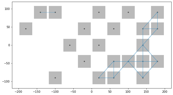
Below we can see that builder selected all the neighbors of order less than equal to 2, with rook contiguity
[21]:
w_rook2 = raster.da2WSP(da_s, "rook", k=2, n_jobs=-1)
splot.plot_spatial_weights(w_rook2, data=da_s)
/opt/anaconda/lib/python3.8/site-packages/scipy/sparse/_index.py:124: SparseEfficiencyWarning: Changing the sparsity structure of a csr_matrix is expensive. lil_matrix is more efficient.
  self._set_arrayXarray(i, j, x)
[21]:
(<Figure size 720x720 with 1 Axes>, <AxesSubplot:>)
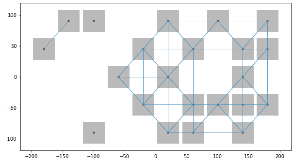
Few times we require the kth order neighbors for our analysis even if lower order neighbors are absent, hence we can use include_nas argument to do the same.
We can also look in both the examples we used n_jobs parameter, and assigned -1 which equats to all the cores present in the computer for multithreading
[22]:
w_rook2 = raster.da2WSP(da_s, "rook", k=2, n_jobs=-1, include_nodata=True)
splot.plot_spatial_weights(w_rook2, data=da_s)
[22]:
(<Figure size 720x720 with 1 Axes>, <AxesSubplot:>)
Additional resources
Dataset links:
[ ]: