This page was generated from user-guide/measure/spatial_polarization.ipynb.
Interactive online version:

Spatial Polarization#
This notebook illustrates the S spatial polarization index implemented in inequality.polarization, based on the graph-intersection framework proposed in:
Rey, S. J. (2026). Mind the gap and the map: measuring distributional and spatial income polarisation. Spatial Economic Analysis. https://doi.org/10.1080/17421772.2025.2606783
Polarization is distinct from inequality: following Esteban and Ray (1994), it combines alienation (how far apart groups are) with group identification (how homogeneous each group is). Zhang and Kanbur (2001) measure spatial polarization as a ratio of between-region to within-region inequality, but require an exogenously fixed partition of space into regions. Rey (2026) instead defines spatial polarization directly from two graphs built over the same set of n locations:
an attribute graph
A, connecting pairs of locations that fall in the same value class (e.g., both above or both below the median of some variable), anda spatial graph
G, connecting pairs of locations that are geographic neighbours.
Intersecting A and G gives a graph I whose edges are pairs that are both attribute-similar and spatially adjacent. Comparing the number of connected components of I, k_I, against k = max(k_A, k_G) and n gives the index:
S(A, G) = 1 - (k_I - k) / (n - k)
S ranges from 0 (no overlap between spatial and attribute structure) to 1 (complete overlap: the connected pieces of the spatial graph line up exactly with the value classes). Splitting the attribute at the median (k=2) gives the spatial bipolarization index; using more than two classes generalizes to spatial multipolarization.
The S class below implements this index and adds a permutation-based inference procedure (randomly reshuffling the attribute values across locations) to obtain a pseudo p-value for the observed statistic - an extension beyond the purely descriptive index presented in the paper, which flags inference as a direction for future work.
[1]:
from inequality.polarization import S
[2]:
import libpysal
import numpy as np
import pandas as pd
from libpysal.graph import Graph
from libpysal.weights import lat2W
A synthetic check: a regular 40x40 lattice#
As a first, controlled example, we place n = 1600 observations on a regular 40x40 lattice (contiguity via lat2W) and assign them the values 0, 1, ..., 1599 in row-major order. Because values increase steadily along each row before dropping back down at the start of the next, splitting at the median (k=2, the default) produces two attribute classes - low and high - that are each spatially contiguous within most rows. We should therefore expect a fairly high, though not perfect,
spatial polarization value.
[3]:
y = np.arange(1600)
[4]:
df = pd.DataFrame({"y": y}, index=y)
[5]:
g = Graph.from_W(lat2W(40, 40))
By default S runs permutations=999 random reshuffles of the attribute values to build a null distribution, so p_value reports how (un)likely the observed spatial polarization would be if the values were randomly scattered across locations instead of following their actual spatial arrangement. n_jobs=4 parallelizes the permutations across four worker processes.
[6]:
res = S(df, g, "y", n_jobs=4)
100%|██████████| 999/999 [00:00<00:00, 1108.24it/s]
[7]:
res
[7]:
S Spatial Polarization Summary
=======================================================
Variable:                                             y
n:                                                 1600
-------------------------------------------------------
S:                                               1.0000
p-value:                                         0.0010
permutations:                                       999
-------------------------------------------------------
Number of attribute components:                       2
Number of spatial components:                         1
Number of intersection components:                    2
=======================================================
Setting permutations=0 skips the inference step entirely and returns just the observed statistic - useful when only the descriptive index is needed, or when many variables are being screened before running significance tests on the interesting ones.
[8]:
res = S(df, g, "y", permutations=0)
0it [00:00, ?it/s]
[9]:
res
[9]:
S Spatial Polarization Summary
=======================================================
Variable:                                             y
n:                                                 1600
-------------------------------------------------------
S:                                               1.0000
-------------------------------------------------------
Number of attribute components:                       2
Number of spatial components:                         1
Number of intersection components:                    2
=======================================================
The labels attribute exposes the underlying classification for every location: a_labels is the attribute (value-class) membership, g_labels the spatial-graph component membership, and i_labels the component membership in the intersection graph I used to compute S.
[10]:
res.labels
[10]:
| i_labels | a_labels | g_labels | |
|---|---|---|---|
| 0 | 0 | 0 | 0 |
| 1 | 0 | 0 | 0 |
| 2 | 0 | 0 | 0 |
| 3 | 0 | 0 | 0 |
| 4 | 0 | 0 | 0 |
| ... | ... | ... | ... |
| 1595 | 1 | 1 | 0 |
| 1596 | 1 | 1 | 0 |
| 1597 | 1 | 1 | 0 |
| 1598 | 1 | 1 | 0 |
| 1599 | 1 | 1 | 0 |
1600 rows × 3 columns
Since permutation inference is embarrassingly parallel, it’s worth checking how much n_jobs helps in practice on this 1,600-observation lattice.
[11]:
%%timeit
res = S(df, g, "y", n_jobs=4)
100%|██████████| 999/999 [00:00<00:00, 5727.70it/s]
100%|██████████| 999/999 [00:00<00:00, 5797.81it/s]
100%|██████████| 999/999 [00:00<00:00, 5759.59it/s]
100%|██████████| 999/999 [00:00<00:00, 5905.86it/s]
100%|██████████| 999/999 [00:00<00:00, 5574.09it/s]
100%|██████████| 999/999 [00:00<00:00, 5774.02it/s]
100%|██████████| 999/999 [00:00<00:00, 5733.33it/s]
100%|██████████| 999/999 [00:00<00:00, 5935.92it/s]
382 ms ± 4.88 ms per loop (mean ± std. dev. of 7 runs, 1 loop each)
For reference, the full source of S - the sparse-graph component counting, quantile binning, and permutation loop - can be inspected directly.
[12]:
S??
Case study: Mexican state income, 1940-2000#
The paper’s illustrative application - reproduced here - examines per-capita GDP for Mexico’s 32 states (31 states plus Ciudad de Mexico) at ten-year intervals from 1940 to 2000. The series extends Esquivel’s (1999) 1940-1990 data with the 2000 figures from Rey and Sastre-Gutierrez (2010), and ships with libpysal.examples as the "mexico" dataset.
Across this 70-year span the distribution of state incomes shows persistent right skew and a pronounced north-south divide, with low-income states concentrated in the south. The question the spatial polarization index is built to answer is not just how unequal incomes are (that’s the job of Theil’s T or the Gini index), but how spatially organized that inequality is - do similarly poor, or similarly rich, states cluster together geographically?
[13]:
libpysal.examples.explain("mexico")
mexico
======

Decennial per capita incomes of Mexican states 1940-2000
--------------------------------------------------------

* mexico.csv: attribute data. (n=32, k=13)
* mexico.gal: spatial weights in GAL format.
* mexicojoin.shp: Polygon shapefile. (n=32)

Data used in Rey, S.J. and M.L. Sastre Gutierrez. (2010) "Interregional inequality dynamics in Mexico." Spatial Economic Analysis, 5: 277-298.
[14]:
mexico = libpysal.examples.load_example("mexico")
[15]:
mexico.get_file_list()
[15]:
['/home/runner/micromamba/envs/test/lib/python3.14/site-packages/libpysal/examples/mexico/mexico.gal',
 '/home/runner/micromamba/envs/test/lib/python3.14/site-packages/libpysal/examples/mexico/mexicojoin.shx',
 '/home/runner/micromamba/envs/test/lib/python3.14/site-packages/libpysal/examples/mexico/mexicojoin.shp',
 '/home/runner/micromamba/envs/test/lib/python3.14/site-packages/libpysal/examples/mexico/mexicojoin.dbf',
 '/home/runner/micromamba/envs/test/lib/python3.14/site-packages/libpysal/examples/mexico/mexico.csv',
 '/home/runner/micromamba/envs/test/lib/python3.14/site-packages/libpysal/examples/mexico/README.md',
 '/home/runner/micromamba/envs/test/lib/python3.14/site-packages/libpysal/examples/mexico/mexicojoin.prj']
[16]:
import geopandas as gpd
[17]:
gdf = gpd.read_file(libpysal.examples.get_path("mexicojoin.shp"))
[18]:
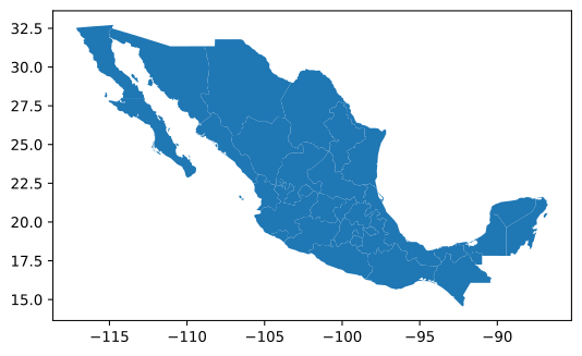
gdf.plot()
[18]:
<Axes: >
[19]:
gdf.head()
[19]:
| POLY_ID | AREA | CODE | NAME | PERIMETER | ACRES | HECTARES | PCGDP1940 | PCGDP1950 | PCGDP1960 | ... | GR9000 | LPCGDP40 | LPCGDP50 | LPCGDP60 | LPCGDP70 | LPCGDP80 | LPCGDP90 | LPCGDP00 | TEST | geometry | |
|---|---|---|---|---|---|---|---|---|---|---|---|---|---|---|---|---|---|---|---|---|---|
| 0 | 1 | 7.252751e+10 | MX02 | Baja California Norte | 2040312.385 | 1.792187e+07 | 7252751.376 | 22361.0 | 20977.0 | 17865.0 | ... | 0.05 | 4.35 | 4.32 | 4.25 | 4.40 | 4.47 | 4.43 | 4.48 | 1.0 | MULTIPOLYGON (((-113.13972 29.01778, -113.2405... |
| 1 | 2 | 7.225988e+10 | MX03 | Baja California Sur | 2912880.772 | 1.785573e+07 | 7225987.769 | 9573.0 | 16013.0 | 16707.0 | ... | 0.00 | 3.98 | 4.20 | 4.22 | 4.39 | 4.46 | 4.41 | 4.42 | 2.0 | MULTIPOLYGON (((-111.20612 25.80278, -111.2302... |
| 2 | 3 | 2.731957e+10 | MX18 | Nayarit | 1034770.341 | 6.750785e+06 | 2731956.859 | 4836.0 | 7515.0 | 7621.0 | ... | -0.05 | 3.68 | 3.88 | 3.88 | 4.04 | 4.13 | 4.11 | 4.06 | 3.0 | MULTIPOLYGON (((-106.62108 21.56531, -106.6475... |
| 3 | 4 | 7.961008e+10 | MX14 | Jalisco | 2324727.436 | 1.967200e+07 | 7961008.285 | 5309.0 | 8232.0 | 9953.0 | ... | 0.03 | 3.73 | 3.92 | 4.00 | 4.21 | 4.32 | 4.30 | 4.33 | 4.0 | POLYGON ((-101.5249 21.85664, -101.5883 21.772... |
| 4 | 5 | 5.467030e+09 | MX01 | Aguascalientes | 313895.530 | 1.350927e+06 | 546702.985 | 10384.0 | 6234.0 | 8714.0 | ... | 0.13 | 4.02 | 3.79 | 3.94 | 4.21 | 4.32 | 4.32 | 4.44 | 5.0 | POLYGON ((-101.8462 22.01176, -101.9653 21.883... |
5 rows × 35 columns
[20]:
S?
The spatial graph G is built from queen contiguity among the 32 states (two states are neighbours if they share at least a boundary point). In the paper this graph is fully connected (k_G = 1), with a density of 13.5%, a median of 4 neighbours per state, ranging from 1 (Baja California Sur) to 9 (San Luis Potosi).
[21]:
sg = Graph.build_contiguity(gdf)
[22]:
sg.n_components
[22]:
1
With k=2 (the default), S splits PCGDP1940 at its median to form the attribute graph - states above the median are mutually “neighbours” in A, as are states below it - and intersects it with the queen contiguity graph. This is the spatial bipolarization index. For 1940, the paper reports a value of 0.87: the low-income states form a single, large connected component running from the southern border up through the centre of the country, while the high-income states are split into
five separate spatial clusters.
[23]:
s1940 = S(gdf, sg, "PCGDP1940")
100%|██████████| 999/999 [00:00<00:00, 3722.73it/s]
[24]:
s1940
[24]:
S Spatial Polarization Summary
=======================================================
Variable:                                     PCGDP1940
n:                                                   32
-------------------------------------------------------
S:                                               0.8667
p-value:                                         0.1310
permutations:                                       999
-------------------------------------------------------
Number of attribute components:                       2
Number of spatial components:                         1
Number of intersection components:                    6
=======================================================
To trace how spatial bipolarization evolves, we repeat the calculation for each decade’s income variable.
[25]:
pcgdp_vars = [f"PCGDP{dec}" for dec in range(1940, 2010, 10)]
[26]:
pcgdp_vars
[26]:
['PCGDP1940',
 'PCGDP1950',
 'PCGDP1960',
 'PCGDP1970',
 'PCGDP1980',
 'PCGDP1990',
 'PCGDP2000']
[27]:
import numpy

rng = numpy.random.default_rng(42)
res = [S(gdf, sg, var) for var in pcgdp_vars]
100%|██████████| 999/999 [00:00<00:00, 3722.67it/s]
100%|██████████| 999/999 [00:00<00:00, 3616.22it/s]
100%|██████████| 999/999 [00:00<00:00, 3535.78it/s]
100%|██████████| 999/999 [00:00<00:00, 3623.66it/s]
100%|██████████| 999/999 [00:00<00:00, 3655.50it/s]
100%|██████████| 999/999 [00:00<00:00, 3437.36it/s]
100%|██████████| 999/999 [00:00<00:00, 3738.29it/s]
[28]:
res[0]
[28]:
S Spatial Polarization Summary
=======================================================
Variable:                                     PCGDP1940
n:                                                   32
-------------------------------------------------------
S:                                               0.8667
p-value:                                         0.1270
permutations:                                       999
-------------------------------------------------------
Number of attribute components:                       2
Number of spatial components:                         1
Number of intersection components:                    6
=======================================================
[29]:
res[1]
[29]:
S Spatial Polarization Summary
=======================================================
Variable:                                     PCGDP1950
n:                                                   32
-------------------------------------------------------
S:                                               0.8667
p-value:                                         0.1020
permutations:                                       999
-------------------------------------------------------
Number of attribute components:                       2
Number of spatial components:                         1
Number of intersection components:                    6
=======================================================
[30]:
res[2]
[30]:
S Spatial Polarization Summary
=======================================================
Variable:                                     PCGDP1960
n:                                                   32
-------------------------------------------------------
S:                                               0.8667
p-value:                                         0.1140
permutations:                                       999
-------------------------------------------------------
Number of attribute components:                       2
Number of spatial components:                         1
Number of intersection components:                    6
=======================================================
[31]:
res[3]
[31]:
S Spatial Polarization Summary
=======================================================
Variable:                                     PCGDP1970
n:                                                   32
-------------------------------------------------------
S:                                               0.9000
p-value:                                         0.0320
permutations:                                       999
-------------------------------------------------------
Number of attribute components:                       2
Number of spatial components:                         1
Number of intersection components:                    5
=======================================================
[32]:
res[4]
[32]:
S Spatial Polarization Summary
=======================================================
Variable:                                     PCGDP1980
n:                                                   32
-------------------------------------------------------
S:                                               0.8333
p-value:                                         0.2780
permutations:                                       999
-------------------------------------------------------
Number of attribute components:                       2
Number of spatial components:                         1
Number of intersection components:                    7
=======================================================
[33]:
res[5]
[33]:
S Spatial Polarization Summary
=======================================================
Variable:                                     PCGDP1990
n:                                                   32
-------------------------------------------------------
S:                                               0.8667
p-value:                                         0.1060
permutations:                                       999
-------------------------------------------------------
Number of attribute components:                       2
Number of spatial components:                         1
Number of intersection components:                    6
=======================================================
[34]:
res[6]
[34]:
S Spatial Polarization Summary
=======================================================
Variable:                                     PCGDP2000
n:                                                   32
-------------------------------------------------------
S:                                               0.8667
p-value:                                         0.1230
permutations:                                       999
-------------------------------------------------------
Number of attribute components:                       2
Number of spatial components:                         1
Number of intersection components:                    6
=======================================================
From bipolarization to multipolarization#
Splitting at the median is just one choice for the attribute graph. Using k>2 quantile classes generalizes the bipolarization index to spatial multipolarization - the same intersection-graph construction, but now A connects locations that fall in the same one of k quantile bins rather than just “above” or “below” the median. Here we repeat the calculation for each decade using tertiles (k=3).
[35]:
res3 = [S(gdf, sg, var, k=3) for var in pcgdp_vars]
100%|██████████| 999/999 [00:00<00:00, 3649.61it/s]
100%|██████████| 999/999 [00:00<00:00, 3559.68it/s]
100%|██████████| 999/999 [00:00<00:00, 3602.58it/s]
100%|██████████| 999/999 [00:00<00:00, 3603.52it/s]
100%|██████████| 999/999 [00:00<00:00, 3467.05it/s]
100%|██████████| 999/999 [00:00<00:00, 3327.73it/s]
100%|██████████| 999/999 [00:00<00:00, 3600.49it/s]
[36]:
for r in res3:
    print(r)
S Spatial Polarization Summary
=======================================================
Variable:                                     PCGDP1940
n:                                                   32
-------------------------------------------------------
S:                                               0.7241
p-value:                                         0.0750
permutations:                                       999
-------------------------------------------------------
Number of attribute components:                       3
Number of spatial components:                         1
Number of intersection components:                   11
=======================================================

S Spatial Polarization Summary
=======================================================
Variable:                                     PCGDP1950
n:                                                   32
-------------------------------------------------------
S:                                               0.8276
p-value:                                         0.0010
permutations:                                       999
-------------------------------------------------------
Number of attribute components:                       3
Number of spatial components:                         1
Number of intersection components:                    8
=======================================================

S Spatial Polarization Summary
=======================================================
Variable:                                     PCGDP1960
n:                                                   32
-------------------------------------------------------
S:                                               0.6897
p-value:                                         0.1560
permutations:                                       999
-------------------------------------------------------
Number of attribute components:                       3
Number of spatial components:                         1
Number of intersection components:                   12
=======================================================

S Spatial Polarization Summary
=======================================================
Variable:                                     PCGDP1970
n:                                                   32
-------------------------------------------------------
S:                                               0.6897
p-value:                                         0.1620
permutations:                                       999
-------------------------------------------------------
Number of attribute components:                       3
Number of spatial components:                         1
Number of intersection components:                   12
=======================================================

S Spatial Polarization Summary
=======================================================
Variable:                                     PCGDP1980
n:                                                   32
-------------------------------------------------------
S:                                               0.6897
p-value:                                         0.1580
permutations:                                       999
-------------------------------------------------------
Number of attribute components:                       3
Number of spatial components:                         1
Number of intersection components:                   12
=======================================================

S Spatial Polarization Summary
=======================================================
Variable:                                     PCGDP1990
n:                                                   32
-------------------------------------------------------
S:                                               0.6552
p-value:                                         0.3000
permutations:                                       999
-------------------------------------------------------
Number of attribute components:                       3
Number of spatial components:                         1
Number of intersection components:                   13
=======================================================

S Spatial Polarization Summary
=======================================================
Variable:                                     PCGDP2000
n:                                                   32
-------------------------------------------------------
S:                                               0.7241
p-value:                                         0.0760
permutations:                                       999
-------------------------------------------------------
Number of attribute components:                       3
Number of spatial components:                         1
Number of intersection components:                   11
=======================================================
More generally, we can sweep over several values of k (bipolar, tertiles, quintiles, septiles) for every decade to see how sensitive the polarization pattern is to the number of attribute classes. Finer classifications (larger k) tend to fragment the attribute graph into more components, which - all else equal - pushes S down, so comparisons across k are best read as “how does the relative ranking across decades change,” rather than as directly comparable magnitudes.
[37]:
res = [S(gdf, sg, var, k=k) for var in pcgdp_vars for k in [2, 3, 5, 7]]
100%|██████████| 999/999 [00:00<00:00, 3731.38it/s]
100%|██████████| 999/999 [00:00<00:00, 3537.63it/s]
100%|██████████| 999/999 [00:00<00:00, 3540.56it/s]
100%|██████████| 999/999 [00:00<00:00, 3689.31it/s]
100%|██████████| 999/999 [00:00<00:00, 3707.63it/s]
100%|██████████| 999/999 [00:00<00:00, 3635.23it/s]
100%|██████████| 999/999 [00:00<00:00, 3480.75it/s]
100%|██████████| 999/999 [00:00<00:00, 3624.50it/s]
100%|██████████| 999/999 [00:00<00:00, 3543.81it/s]
100%|██████████| 999/999 [00:00<00:00, 3534.07it/s]
100%|██████████| 999/999 [00:00<00:00, 3598.41it/s]
100%|██████████| 999/999 [00:00<00:00, 3780.01it/s]
100%|██████████| 999/999 [00:00<00:00, 3544.62it/s]
100%|██████████| 999/999 [00:00<00:00, 3576.05it/s]
100%|██████████| 999/999 [00:00<00:00, 3411.04it/s]
100%|██████████| 999/999 [00:00<00:00, 3353.64it/s]
100%|██████████| 999/999 [00:00<00:00, 3703.79it/s]
100%|██████████| 999/999 [00:00<00:00, 3657.12it/s]
100%|██████████| 999/999 [00:00<00:00, 3500.54it/s]
100%|██████████| 999/999 [00:00<00:00, 3756.92it/s]
100%|██████████| 999/999 [00:00<00:00, 3508.19it/s]
100%|██████████| 999/999 [00:00<00:00, 3558.39it/s]
100%|██████████| 999/999 [00:00<00:00, 3558.65it/s]
100%|██████████| 999/999 [00:00<00:00, 3645.21it/s]
100%|██████████| 999/999 [00:00<00:00, 3567.02it/s]
100%|██████████| 999/999 [00:00<00:00, 3541.21it/s]
100%|██████████| 999/999 [00:00<00:00, 3661.45it/s]
100%|██████████| 999/999 [00:00<00:00, 3612.39it/s]
[38]:
for r in res:
    print(r)
S Spatial Polarization Summary
=======================================================
Variable: PCGDP1940
n: 32
-------------------------------------------------------
S: 0.8667
p-value: 0.1160
permutations: 999
-------------------------------------------------------
Number of attribute components: 2
Number of spatial components: 1
Number of intersection components: 6
=======================================================
S Spatial Polarization Summary
=======================================================
Variable: PCGDP1940
n: 32
-------------------------------------------------------
S: 0.7241
p-value: 0.0580
permutations: 999
-------------------------------------------------------
Number of attribute components: 3
Number of spatial components: 1
Number of intersection components: 11
=======================================================
S Spatial Polarization Summary
=======================================================
Variable: PCGDP1940
n: 32
-------------------------------------------------------
S: 0.6667
p-value: 0.0010
permutations: 999
-------------------------------------------------------
Number of attribute components: 5
Number of spatial components: 1
Number of intersection components: 14
=======================================================
S Spatial Polarization Summary
=======================================================
Variable: PCGDP1940
n: 32
-------------------------------------------------------
S: 0.3600
p-value: 0.2580
permutations: 999
-------------------------------------------------------
Number of attribute components: 7
Number of spatial components: 1
Number of intersection components: 23
=======================================================
S Spatial Polarization Summary
=======================================================
Variable: PCGDP1950
n: 32
-------------------------------------------------------
S: 0.8667
p-value: 0.1100
permutations: 999
-------------------------------------------------------
Number of attribute components: 2
Number of spatial components: 1
Number of intersection components: 6
=======================================================
S Spatial Polarization Summary
=======================================================
Variable: PCGDP1950
n: 32
-------------------------------------------------------
S: 0.8276
p-value: 0.0030
permutations: 999
-------------------------------------------------------
Number of attribute components: 3
Number of spatial components: 1
Number of intersection components: 8
=======================================================
S Spatial Polarization Summary
=======================================================
Variable: PCGDP1950
n: 32
-------------------------------------------------------
S: 0.7037
p-value: 0.0010
permutations: 999
-------------------------------------------------------
Number of attribute components: 5
Number of spatial components: 1
Number of intersection components: 13
=======================================================
S Spatial Polarization Summary
=======================================================
Variable: PCGDP1950
n: 32
-------------------------------------------------------
S: 0.4400
p-value: 0.0760
permutations: 999
-------------------------------------------------------
Number of attribute components: 7
Number of spatial components: 1
Number of intersection components: 21
=======================================================
S Spatial Polarization Summary
=======================================================
Variable: PCGDP1960
n: 32
-------------------------------------------------------
S: 0.8667
p-value: 0.1090
permutations: 999
-------------------------------------------------------
Number of attribute components: 2
Number of spatial components: 1
Number of intersection components: 6
=======================================================
S Spatial Polarization Summary
=======================================================
Variable: PCGDP1960
n: 32
-------------------------------------------------------
S: 0.6897
p-value: 0.1530
permutations: 999
-------------------------------------------------------
Number of attribute components: 3
Number of spatial components: 1
Number of intersection components: 12
=======================================================
S Spatial Polarization Summary
=======================================================
Variable: PCGDP1960
n: 32
-------------------------------------------------------
S: 0.4815
p-value: 0.2020
permutations: 999
-------------------------------------------------------
Number of attribute components: 5
Number of spatial components: 1
Number of intersection components: 19
=======================================================
S Spatial Polarization Summary
=======================================================
Variable: PCGDP1960
n: 32
-------------------------------------------------------
S: 0.2800
p-value: 0.6320
permutations: 999
-------------------------------------------------------
Number of attribute components: 7
Number of spatial components: 1
Number of intersection components: 25
=======================================================
S Spatial Polarization Summary
=======================================================
Variable: PCGDP1970
n: 32
-------------------------------------------------------
S: 0.9000
p-value: 0.0340
permutations: 999
-------------------------------------------------------
Number of attribute components: 2
Number of spatial components: 1
Number of intersection components: 5
=======================================================
S Spatial Polarization Summary
=======================================================
Variable: PCGDP1970
n: 32
-------------------------------------------------------
S: 0.6897
p-value: 0.1420
permutations: 999
-------------------------------------------------------
Number of attribute components: 3
Number of spatial components: 1
Number of intersection components: 12
=======================================================
S Spatial Polarization Summary
=======================================================
Variable: PCGDP1970
n: 32
-------------------------------------------------------
S: 0.4444
p-value: 0.3580
permutations: 999
-------------------------------------------------------
Number of attribute components: 5
Number of spatial components: 1
Number of intersection components: 20
=======================================================
S Spatial Polarization Summary
=======================================================
Variable: PCGDP1970
n: 32
-------------------------------------------------------
S: 0.3200
p-value: 0.4540
permutations: 999
-------------------------------------------------------
Number of attribute components: 7
Number of spatial components: 1
Number of intersection components: 24
=======================================================
S Spatial Polarization Summary
=======================================================
Variable: PCGDP1980
n: 32
-------------------------------------------------------
S: 0.8333
p-value: 0.2660
permutations: 999
-------------------------------------------------------
Number of attribute components: 2
Number of spatial components: 1
Number of intersection components: 7
=======================================================
S Spatial Polarization Summary
=======================================================
Variable: PCGDP1980
n: 32
-------------------------------------------------------
S: 0.6897
p-value: 0.1400
permutations: 999
-------------------------------------------------------
Number of attribute components: 3
Number of spatial components: 1
Number of intersection components: 12
=======================================================
S Spatial Polarization Summary
=======================================================
Variable: PCGDP1980
n: 32
-------------------------------------------------------
S: 0.4074
p-value: 0.5060
permutations: 999
-------------------------------------------------------
Number of attribute components: 5
Number of spatial components: 1
Number of intersection components: 21
=======================================================
S Spatial Polarization Summary
=======================================================
Variable: PCGDP1980
n: 32
-------------------------------------------------------
S: 0.3600
p-value: 0.2740
permutations: 999
-------------------------------------------------------
Number of attribute components: 7
Number of spatial components: 1
Number of intersection components: 23
=======================================================
S Spatial Polarization Summary
=======================================================
Variable: PCGDP1990
n: 32
-------------------------------------------------------
S: 0.8667
p-value: 0.1150
permutations: 999
-------------------------------------------------------
Number of attribute components: 2
Number of spatial components: 1
Number of intersection components: 6
=======================================================
S Spatial Polarization Summary
=======================================================
Variable: PCGDP1990
n: 32
-------------------------------------------------------
S: 0.6552
p-value: 0.2750
permutations: 999
-------------------------------------------------------
Number of attribute components: 3
Number of spatial components: 1
Number of intersection components: 13
=======================================================
S Spatial Polarization Summary
=======================================================
Variable: PCGDP1990
n: 32
-------------------------------------------------------
S: 0.5185
p-value: 0.0790
permutations: 999
-------------------------------------------------------
Number of attribute components: 5
Number of spatial components: 1
Number of intersection components: 18
=======================================================
S Spatial Polarization Summary
=======================================================
Variable: PCGDP1990
n: 32
-------------------------------------------------------
S: 0.4400
p-value: 0.0480
permutations: 999
-------------------------------------------------------
Number of attribute components: 7
Number of spatial components: 1
Number of intersection components: 21
=======================================================
S Spatial Polarization Summary
=======================================================
Variable: PCGDP2000
n: 32
-------------------------------------------------------
S: 0.8667
p-value: 0.1100
permutations: 999
-------------------------------------------------------
Number of attribute components: 2
Number of spatial components: 1
Number of intersection components: 6
=======================================================
S Spatial Polarization Summary
=======================================================
Variable: PCGDP2000
n: 32
-------------------------------------------------------
S: 0.7241
p-value: 0.0600
permutations: 999
-------------------------------------------------------
Number of attribute components: 3
Number of spatial components: 1
Number of intersection components: 11
=======================================================
S Spatial Polarization Summary
=======================================================
Variable: PCGDP2000
n: 32
-------------------------------------------------------
S: 0.4444
p-value: 0.3460
permutations: 999
-------------------------------------------------------
Number of attribute components: 5
Number of spatial components: 1
Number of intersection components: 20
=======================================================
S Spatial Polarization Summary
=======================================================
Variable: PCGDP2000
n: 32
-------------------------------------------------------
S: 0.3200
p-value: 0.4450
permutations: 999
-------------------------------------------------------
Number of attribute components: 7
Number of spatial components: 1
Number of intersection components: 24
=======================================================
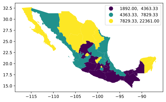
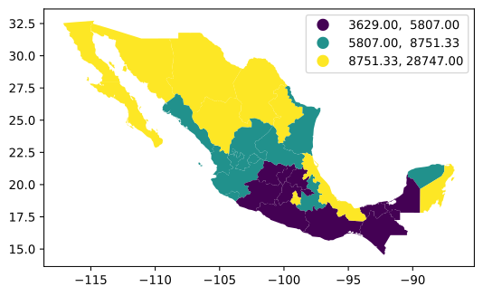
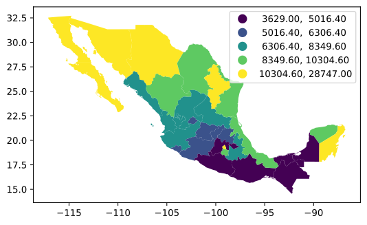
It helps to look at the actual quantile classifications behind these numbers before interpreting the index values.
[39]:
gdf.plot("PCGDP1940", scheme="quantiles", k=3, legend=True)
[39]:
<Axes: >
[40]:
gdf.plot("PCGDP1950", scheme="quantiles", k=3, legend=True)
[40]:
<Axes: >
[41]:
gdf.plot("PCGDP1950", scheme="quantiles", k=5, legend=True)
[41]:
<Axes: >
Beyond the summary statistic, an S object exposes the full component bookkeeping behind it: the number of components in the intersection, spatial, and attribute graphs, and the per-location labels used to build them.
[42]:
res[-1].n_i_components
[42]:
24
[43]:
res[-1].labels
[43]:
| i_labels | a_labels | g_labels | |
|---|---|---|---|
| 0 | 0 | 5 | 0 |
| 1 | 1 | 4 | 0 |
| 2 | 2 | 0 | 0 |
| 3 | 3 | 4 | 0 |
| 4 | 4 | 5 | 0 |
| 5 | 5 | 2 | 0 |
| 6 | 6 | 5 | 0 |
| 7 | 7 | 1 | 0 |
| 8 | 8 | 1 | 0 |
| 9 | 9 | 3 | 0 |
| 10 | 10 | 6 | 0 |
| 11 | 3 | 4 | 0 |
| 12 | 9 | 3 | 0 |
| 13 | 11 | 3 | 0 |
| 14 | 12 | 6 | 0 |
| 15 | 13 | 2 | 0 |
| 16 | 12 | 6 | 0 |
| 17 | 14 | 0 | 0 |
| 18 | 8 | 1 | 0 |
| 19 | 15 | 0 | 0 |
| 20 | 16 | 2 | 0 |
| 21 | 15 | 0 | 0 |
| 22 | 17 | 4 | 0 |
| 23 | 18 | 6 | 0 |
| 24 | 19 | 5 | 0 |
| 25 | 20 | 2 | 0 |
| 26 | 21 | 3 | 0 |
| 27 | 2 | 0 | 0 |
| 28 | 5 | 2 | 0 |
| 29 | 22 | 6 | 0 |
| 30 | 23 | 4 | 0 |
| 31 | 7 | 1 | 0 |
[44]:
r0 = res[-1]
[45]:
dir(r0)
[45]:
['__class__',
 '__delattr__',
 '__dict__',
 '__dir__',
 '__doc__',
 '__eq__',
 '__firstlineno__',
 '__format__',
 '__ge__',
 '__getattribute__',
 '__getstate__',
 '__gt__',
 '__hash__',
 '__init__',
 '__init_subclass__',
 '__le__',
 '__lt__',
 '__module__',
 '__ne__',
 '__new__',
 '__reduce__',
 '__reduce_ex__',
 '__repr__',
 '__setattr__',
 '__sizeof__',
 '__static_attributes__',
 '__str__',
 '__subclasshook__',
 '__weakref__',
 'column',
 'labels',
 'n',
 'n_a_components',
 'n_g_components',
 'n_i_components',
 'p_value',
 'permutations',
 'statistic_']
[46]:
r0.permutations
[46]:
999
[47]:
r0.statistic_
[47]:
0.31999999999999995
[48]:
r0.p_value
[48]:
np.float64(0.445)
Comparing polarization across decades and classification schemes#
Putting it together, we compute the index, its Monte Carlo p-value, and the number of intersection components for every combination of k in [2, 3, 5, 7] and decade, and collect the results into a single dataframe for comparison - in the same spirit as the paper’s comparison of the spatial polarization trajectory against Theil’s T over time.
[49]:
rng = numpy.random.default_rng(42)

res = []
for k in [2, 3, 5, 7]:
    for year in [1940, 1950, 1960, 1970, 1980, 1990, 2000]:
        v = f"PCGDP{year}"
        r = S(gdf, sg, v, k=k)
        res.append([year, k, r.statistic_, r.p_value, r.n_i_components])
100%|██████████| 999/999 [00:00<00:00, 3670.72it/s]
100%|██████████| 999/999 [00:00<00:00, 3450.03it/s]
100%|██████████| 999/999 [00:00<00:00, 3699.55it/s]
100%|██████████| 999/999 [00:00<00:00, 3665.62it/s]
100%|██████████| 999/999 [00:00<00:00, 3471.00it/s]
100%|██████████| 999/999 [00:00<00:00, 3622.54it/s]
100%|██████████| 999/999 [00:00<00:00, 3739.26it/s]
100%|██████████| 999/999 [00:00<00:00, 3624.68it/s]
100%|██████████| 999/999 [00:00<00:00, 3703.41it/s]
100%|██████████| 999/999 [00:00<00:00, 3697.94it/s]
100%|██████████| 999/999 [00:00<00:00, 3775.71it/s]
100%|██████████| 999/999 [00:00<00:00, 3673.84it/s]
100%|██████████| 999/999 [00:00<00:00, 3597.51it/s]
100%|██████████| 999/999 [00:00<00:00, 3734.26it/s]
100%|██████████| 999/999 [00:00<00:00, 3594.20it/s]
100%|██████████| 999/999 [00:00<00:00, 3638.10it/s]
100%|██████████| 999/999 [00:00<00:00, 3425.69it/s]
100%|██████████| 999/999 [00:00<00:00, 3460.10it/s]
100%|██████████| 999/999 [00:00<00:00, 3644.66it/s]
100%|██████████| 999/999 [00:00<00:00, 3643.82it/s]
100%|██████████| 999/999 [00:00<00:00, 3619.74it/s]
100%|██████████| 999/999 [00:00<00:00, 3612.30it/s]
100%|██████████| 999/999 [00:00<00:00, 3804.28it/s]
100%|██████████| 999/999 [00:00<00:00, 3682.79it/s]
100%|██████████| 999/999 [00:00<00:00, 3397.71it/s]
100%|██████████| 999/999 [00:00<00:00, 3644.21it/s]
100%|██████████| 999/999 [00:00<00:00, 3457.93it/s]
100%|██████████| 999/999 [00:00<00:00, 3725.95it/s]
[50]:
import pandas as pd
[51]:
res_df = pd.DataFrame(data=np.array(res), columns=["year", "k", "s", "p", "n_i"])
[52]:
res_df.head()
[52]:
| year | k | s | p | n_i | |
|---|---|---|---|---|---|
| 0 | 1940.0 | 2.0 | 0.866667 | 0.089 | 6.0 |
| 1 | 1950.0 | 2.0 | 0.866667 | 0.105 | 6.0 |
| 2 | 1960.0 | 2.0 | 0.866667 | 0.113 | 6.0 |
| 3 | 1970.0 | 2.0 | 0.900000 | 0.026 | 5.0 |
| 4 | 1980.0 | 2.0 | 0.833333 | 0.293 | 7.0 |
Filtering to the statistically significant results (p <= 0.05 under the permutation null) highlights which decade/classification combinations show spatial polarization stronger than would be expected if incomes were randomly scattered across the map rather than concentrated by geography.
[53]:
res_df[res_df.p <= 0.05]
[53]:
| year | k | s | p | n_i | |
|---|---|---|---|---|---|
| 3 | 1970.0 | 2.0 | 0.900000 | 0.026 | 5.0 |
| 8 | 1950.0 | 3.0 | 0.827586 | 0.003 | 8.0 |
| 14 | 1940.0 | 5.0 | 0.666667 | 0.001 | 14.0 |
| 15 | 1950.0 | 5.0 | 0.703704 | 0.001 | 13.0 |
[54]:
res_df[res_df.year == 2000]
[54]:
| year | k | s | p | n_i | |
|---|---|---|---|---|---|
| 6 | 2000.0 | 2.0 | 0.866667 | 0.115 | 6.0 |
| 13 | 2000.0 | 3.0 | 0.724138 | 0.072 | 11.0 |
| 20 | 2000.0 | 5.0 | 0.444444 | 0.328 | 20.0 |
| 27 | 2000.0 | 7.0 | 0.320000 | 0.447 | 24.0 |
Summary#
Across both the synthetic lattice and the Mexican states application, S quantifies something inequality measures like the Gini index or Theil’s T cannot: whether similar values are organized in space. As Rey (2026) shows for Mexico, national income inequality (Theil’s T) and spatial polarization can move independently - inequality between states can fall even while the geographic clustering of rich and poor states persists or intensifies, consistent with a persistent poverty trap in the
south alongside a more spatially fragmented set of high-income states elsewhere in the country.