
What if you want to calculate the best segregation measure starting with no data?
We've got you covered
This notebook uses functionality found in the cenpy.products module, which will be released officially in July. If you want to replicate this notebook prior to cenpy's 1.0 release, you can install the development version of with pip install git+https://github.com/ljwolf/cenpy.git@product
Further, the notebook leverages a function from contextily that has not yet been released. Similar to above, you can use the most recent github version of the library to replicated the functionality in this notebook with pip install git+https://github.com/darribas/contextily.git
%load_ext autoreload
%autoreload 2
import geopandas as gpd
import segregation
import matplotlib.pyplot as plt
import seaborn as sns
import contextily as ctx
import cenpy

sns.set_context('notebook')
cenpy.set_sitekey('d4d0ad648fffc219dc272b6af90e5b2106235a12', overwrite=True) # note you should replace this key with your own from here: https://api.census.gov/data/key_signup.html
First, we need to collect some data from the Census API. Using cenpy, we can grab all the necessary data in a single call. Let's store the variables we need in a list (these are total population counts from the 2017 ACS. See the census api docs for more details)
black = 'B03002_004E'
white = 'B03002_003E'
hispanic = 'B03002_012E'
asian = 'B03002_006E'
variables = [white, black, hispanic, asian]
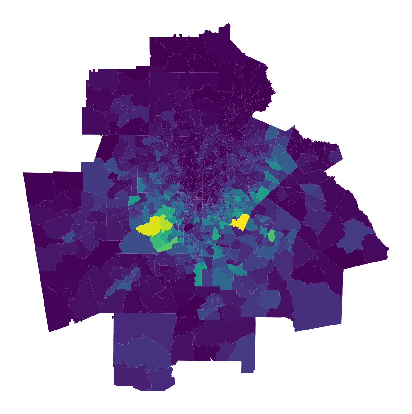
Using Atlanta as a test case, we'll grab the data for the four different race categories and plot the non-hispanic Black population
atl = cenpy.products.ACS(2017).from_msa(name='Atlanta, GA', variables=variables.copy(), level='tract')
atl.head()
fig, ax = plt.subplots(1,1, figsize=(12,12))
atl.plot(column='B03002_004E', ax=ax)
ax.axis('off')
atl = atl.to_crs({'init': 'epsg:4326'})
Now, we'll grab a walkable street network from OSM and use it to calculate our distance-decayed population sums. Under the hood we're using pandana and urbanaccess from the wonderful UDST
atl_network = segregation.network.get_osm_network(atl)
downloading the network takes awhile, so uncomment to save it and you can load later
# atl_network.save_hdf5('atl_network.h5')
and use this to read it back in
import pandana as pdna
atl_network = pdna.Network.from_hdf5('atl_network.h5')
# Note that the most recent version of pandana may have some issues with memory consumption that could lead to failure (https://github.com/UDST/pandana/issues/107)
# If your kernel crashes running this cell, try setting a smaller threshold distance like 1000

# this cell can also take

atl_access = segregation.network.calc_access(atl, network=atl_network, distance=5000, decay='exp', variables=variables)
atl_access.head()
Inside the accessibility calculation, pandana is snapping each tract centroid to its nearest intersection on the walk network. Then, it calculates the shortest path distance between every pair of intersrctions in the network and sums up the total population for each group accessible within the specified threshold, while applying a distance decay function to discount further distances
That means population access is measured for each intersection in the network. In essence, we're modeling down from the tract level to the intersection level. We can quickly convert the network intersections to a geopandas GeoDataFrame to plot and compare with the original tracts
net_points =gpd.GeoDataFrame(atl_access, geometry=gpd.points_from_xy(atl_network.nodes_df['x'],atl_network.nodes_df['y']))
net_points.crs = {'init': 'epsg:4326'}
fig, ax = plt.subplots(1,2,figsize=(30,15))


# tracts
atl.to_crs({'init': 'epsg:3857'}).plot('B03002_004E', ax=ax[0], cmap='magma')
ctx.add_basemap(ax[0],url=ctx.sources.ST_TONER_LITE)
ax[0].axis('off')
ax[0].set_title('Original Tract-Level Data',fontsize=24)

# network
net_points[net_points.acc_B03002_004E > 0].to_crs({'init': 'epsg:3857'}).plot('acc_B03002_004E', alpha=0.01, ax=ax[1], cmap='magma', s=20)
ctx.add_basemap(ax[1],url=ctx.sources.ST_TONER_LITE )
ax[1].axis('off')
ax[1].set_title('Intersection-Level Accessibility Surface ', fontsize=24)

plt.suptitle('Non-Hispanic Black Population')
plt.tight_layout()
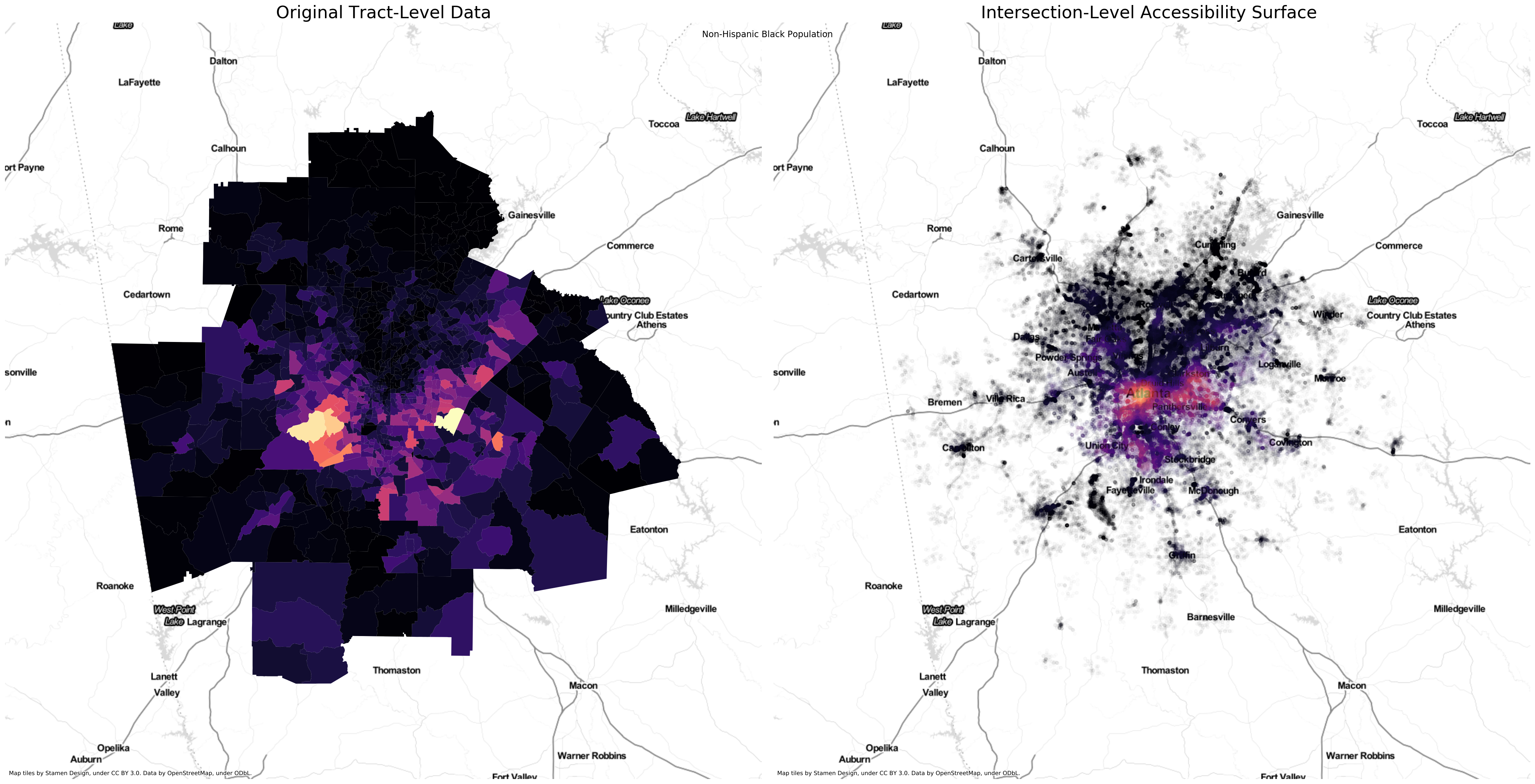
The main advantage of the plot on the right
is that we avoid the visual distortion created by the large but sparsely populated tracts on the periphery and between the highways. It's a much better representation of metropolitan Atlanta's spatial structure. We use this version to compute the spatial information theory index.
Apart from the fact that we're now constraining the visualization to only the developed land, using transparency gives a further sense of the metro's development intensity, since denser areas appear more saturated. The hues have shifted in space slightly (e.g. the the brightest locus has shifted from the southwest in the left map toward the center in the right map) since they now represent distance-weighted densities, rather than totals.
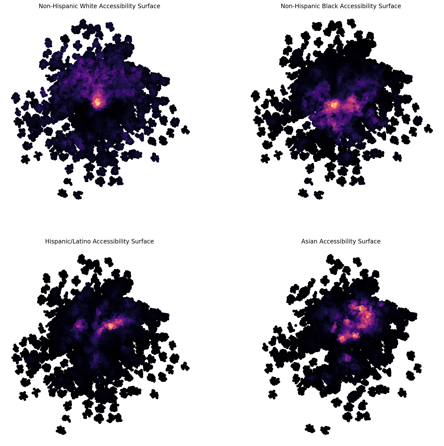
fig, ax = plt.subplots(2,2, figsize=(16,16))
ax = ax.flatten()


net_points[net_points.acc_B03002_003E > 0].to_crs({'init': 'epsg:3857'}).plot('acc_B03002_003E', ax=ax[0], cmap='magma', s=20)
#ctx.add_basemap(ax[1],url=ctx.sources.ST_TONER_LITE )
ax[0].axis('off')
ax[0].set_title('Non-Hispanic White Accessibility Surface ')

net_points[net_points.acc_B03002_004E > 0].to_crs({'init': 'epsg:3857'}).plot('acc_B03002_004E', ax=ax[1], cmap='magma', s=20)
#ctx.add_basemap(ax[1],url=ctx.sources.ST_TONER_LITE )
ax[1].axis('off')
ax[1].set_title('Non-Hispanic Black Accessibility Surface ')

net_points[net_points.acc_B03002_012E > 0].to_crs({'init': 'epsg:3857'}).plot('acc_B03002_012E', ax=ax[2], cmap='magma', s=20)
#ctx.add_basemap(ax[1],url=ctx.sources.ST_TONER_LITE )
ax[2].axis('off')
ax[2].set_title('Hispanic/Latino Accessibility Surface ')

net_points[net_points.acc_B03002_006E > 0].to_crs({'init': 'epsg:3857'}).plot('acc_B03002_006E', ax=ax[3], cmap='magma', s=20)
#ctx.add_basemap(ax[1],url=ctx.sources.ST_TONER_LITE )
ax[3].axis('off')
ax[3].set_title('Asian Accessibility Surface ')
Now we can use these surfaces to calculate the multi-group network-based spatial information theory index
from segregation.aspatial import Multi_Information_Theory
accvars = ['acc_'+variable for variable in variables]
# spatial information theory using the network kernel

Multi_Information_Theory(atl_access, accvars).statistic
We can compare this statistic with what we would obtain if we didn't consider spatial effects (i.e. if local context is only considered the census tract itself)
# aspatial information theory

Multi_Information_Theory((atl, variables).statistic