
Quadrat Based Statistical Method for Planar Point Patterns
Authors: Serge Rey sjsrey@gmail.com, Wei Kang weikang9009@gmail.com and Hu Shao shaohutiger@gmail.com
Introduction
In this notebook, we are going to introduce how to apply quadrat statistics to a point pattern to infer whether it comes from a CSR process.
- In Quadrat Statistic we introduce the concept of quadrat based method.
- We illustrate how to use the module quadrat_statistics.py through an example dataset juvenile in Juvenile Example
Quadrat Statistic
In the previous notebooks, we introduced the concept of Complete Spatial Randomness (CSR) process which serves as the benchmark process. Utilizing CSR properties, we can discriminate those that are not from a CSR process. Quadrat statistic is one such method. Since a CSR process has two major characteristics:
- Uniform: each location has equal probability of getting a point (where an event happens).
- Independent: location of event points are independent.
We can imagine that for any point pattern, if the underlying process is a CSR process, the expected point counts inside any cell of area $|A|$ should be $\lambda |A|$ ($\lambda$ is the intensity which is uniform across the study area for a CSR). Thus, if we impose a $m \times k$ rectangular tessellation over the study area (window), we can easily calculate the expected number of points inside each cell under the null of CSR. By comparing the observed point counts against the expected counts and calculate a $\chi^2$ test statistic, we can decide whether to reject the null based on the position of the $\chi^2$ test statistic in the sampling distribution.
$$\chi^2 = \sum^m_{i=1} \sum^k_{j=1} \frac{[x_{i,j}-E(x_{i,j})]^2}{\lambda |A_{i,j}|}$$There are two ways to construct the sampling distribution and acquire a p-value:
- Analytical sampling distribution: a $\chi^2$ distribution of $m \times k -1$ degree of freedom. We can refer to the $\chi^2$ distribution table to acquire the p-value. If it is smaller than $0.05$, we will reject the null at the $95\%$ confidence level.
- Empirical sampling distribution: a distribution constructed from a large number of $\chi^2$ test statistics for simulations under the null of CSR. If the $\chi^2$ test statistic for the observed point pattern is among the largest $5%$ test statistics, we would say that it is very unlikely that it is the outcome of a CSR process at the $95\%$ confidence level. Then, the null is rejected. A pseudo p-value can be calculated based on which we can use the same rule as p-value to make the decision: $$p(\chi^2) = \frac{1+\sum^{nsim}_{i=1}\phi_i}{nsim+1}$$ where $$ \phi_i = \begin{cases} 1 & \quad \text{if } \psi_i^2 \geq \chi^2 \\ 0 & \quad \text{otherwise } \\ \end{cases} $$
$nsim$ is the number of simulations, $\psi_i^2$ is the $\chi^2$ test statistic calculated for each simulated point pattern, $\chi^2$ is the $\chi^2$ test statistic calculated for the observed point pattern, $\phi_i$ is an indicator variable.
We are going to introduce how to use the quadrat_statistics.py module to perform quadrat based method using either of the above two approaches to constructing the sampling distribution and acquire a p-value.
import libpysal as ps
import numpy as np
from pointpats import PointPattern, as_window
from pointpats import PoissonPointProcess as csr
%matplotlib inline
import matplotlib.pyplot as plt
Import the quadrat_statistics module to conduct quadrat-based method.
Among the three major classes in the module, RectangleM, HexagonM, QStatistic, the first two are aimed at imposing a tessellation (rectangular or hexagonal shape) over the minimum bounding rectangle of the point pattern and calculate the number of points falling in each cell; QStatistic is the main class with which we can calculate a p-value, as well as a pseudo p-value to help us make the decision of rejecting the null or not.
import pointpats.quadrat_statistics as qs
dir(qs)
Open the point shapefile "juvenile.shp".
juv = ps.io.open(ps.examples.get_path("juvenile.shp"))
len(juv) # 168 point events in total
juv_points = np.array([event for event in juv]) # get x,y coordinates for all the points
juv_points
Construct a point pattern from numpy array juv_points.
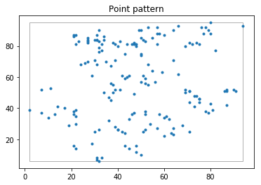
pp_juv = PointPattern(juv_points)
pp_juv
pp_juv.summary()
pp_juv.plot(window= True, title= "Point pattern")
q_r = qs.QStatistic(pp_juv,shape= "rectangle",nx = 3, ny = 3)
Use the plot method to plot the quadrats as well as the number of points falling in each quadrat.
q_r.plot()
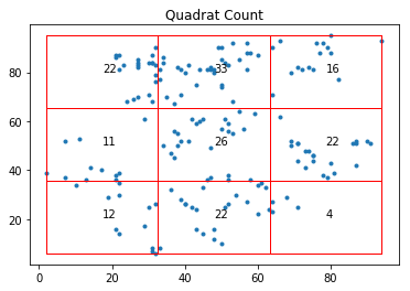
q_r.chi2 #chi-squared test statistic for the observed point pattern
q_r.df #degree of freedom
q_r.chi2_pvalue # analytical pvalue
Since the p-value based on the analytical $\chi^2$ distribution (degree of freedom = 8) is 0.0000589, much smaller than 0.05. We might determine that the underlying process is not CSR. We can also turn to empirical sampling distribution to ascertain our decision.
csr_process = csr(pp_juv.window, pp_juv.n, 999, asPP=True)
We specify parameter realizations as the point process instance which contains 999 CSR realizations.
q_r_e = qs.QStatistic(pp_juv,shape= "rectangle",nx = 3, ny = 3, realizations = csr_process)
q_r_e.chi2_r_pvalue
The pseudo p-value is 0.002, which is smaller than 0.05. Thus, we reject the null at the $95\%$ confidence level.
q_h = qs.QStatistic(pp_juv,shape= "hexagon",lh = 15)
q_h.plot()
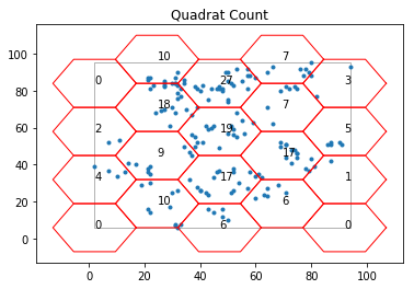
q_h.chi2 #chi-squared test statistic for the observed point pattern
q_h.df #degree of freedom
q_h.chi2_pvalue # analytical pvalue
Similar to the inference of rectangle tessellation, since the analytical p-value is much smaller than 0.05, we reject the null of CSR. The point pattern is not random.
q_h_e = qs.QStatistic(pp_juv,shape= "hexagon",lh = 15, realizations = csr_process)
q_h_e.chi2_r_pvalue
Because 0.001 is smaller than 0.05, we reject the null.